The Growth of Functions

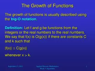
1. The Growth of Functions • The growth of functions is usually described using the big-O notation. • Definition: Let f and g be functions from the integers or the real numbers to the real numbers. • We say that f(x) is O(g(x)) if there are constants C and k such that • |f(x)|  C|g(x)| • whenever x > k. Applied Discrete Mathematics Week 3: Algorithms

2. The Growth of Functions • When we analyze the growth of complexity functions, f(x) and g(x) are always positive. • Therefore, we can simplify the big-O requirement to • f(x)  Cg(x) whenever x > k. • If we want to show that f(x) is O(g(x)), we only need to find one pair (C, k) (which is never unique). Applied Discrete Mathematics Week 3: Algorithms

3. The Growth of Functions • The idea behind the big-O notation is to establish an upper boundary for the growth of a function f(x) for large x. • This boundary is specified by a function g(x) that is usually much simpler than f(x). • We accept the constant C in the requirement • f(x)  Cg(x) whenever x > k, • because C does not grow with x. • We are only interested in large x, so it is OK iff(x) > Cg(x) for x  k. Applied Discrete Mathematics Week 3: Algorithms

4. The Growth of Functions • Example: • Show that f(x) = x2 + 2x + 1 is O(x2). • For x > 1 we have: • x2 + 2x + 1  x2 + 2x2 + x2 •  x2 + 2x + 1  4x2 • Therefore, for C = 4 and k = 1: • f(x)  Cx2 whenever x > k. •  f(x) is O(x2). Applied Discrete Mathematics Week 3: Algorithms

5. The Growth of Functions • Question: If f(x) is O(x2), is it also O(x3)? • Yes. x3 grows faster than x2, so x3 grows also faster than f(x). • Therefore, we always have to find the smallest simple function g(x) for which f(x) is O(g(x)). Applied Discrete Mathematics Week 3: Algorithms

6. The Growth of Functions • “Popular” functions g(n) are • n log n, 1, 2n, n2, n!, n, n3, log n • Listed from slowest to fastest growth: • 1 • log n • n • n log n • n2 • n3 • 2n • n! Applied Discrete Mathematics Week 3: Algorithms

7. The Growth of Functions • A problem that can be solved with polynomial worst-case complexity is called tractable. • Problems of higher complexity are called intractable. • Problems that no algorithm can solve are called unsolvable. • You will find out more about this in CS420. Applied Discrete Mathematics Week 3: Algorithms

8. Useful Rules for Big-O • For any polynomial f(x) = anxn + an-1xn-1 + … + a0, where a0, a1, …, an are real numbers, • f(x) is O(xn). • If f1(x) is O(g(x)) and f2(x) is O(g(x)), then(f1 + f2)(x) is O(g(x)). • If f1(x) is O(g1(x)) and f2(x) is O(g2(x)), then (f1 + f2)(x) is O(max(g1(x), g2(x))) • If f1(x) is O(g1(x)) and f2(x) is O(g2(x)), then (f1f2)(x) is O(g1(x) g2(x)). Applied Discrete Mathematics Week 3: Algorithms

9. Complexity Examples • What does the following algorithm compute? • procedurewho_knows(a1, a2, …, an: integers) • who_knows := 0 • fori := 1 to n-1 • for j := i+1 to n • if |ai – aj| > who_knowsthenwho_knows := |ai – aj| • {who_knows is the maximum difference between any two numbers in the input sequence} • Comparisons: n-1 + n-2 + n-3 + … + 1 • = (n – 1)n/2 = 0.5n2 – 0.5n • Time complexity is O(n2). Applied Discrete Mathematics Week 3: Algorithms

10. Complexity Examples • Another algorithm solving the same problem: • proceduremax_diff(a1, a2, …, an: integers) • min := a1 • max := a1 • fori := 2 to n • ifai < min then min := ai • else if ai > max then max := ai • max_diff := max - min • Comparisons (worst case): 2n - 2 • Time complexity is O(n). Applied Discrete Mathematics Week 3: Algorithms

11. Let us talk about… • Predicate Calculus … so that you can understand Assignment #1 better. Applied Discrete Mathematics Week 3: Algorithms

12. Propositional Functions • Propositional function (open sentence): • statement involving one or more variables, • e.g.: x-3 > 5. • Let us call this propositional function P(x), where P is the predicate and x is the variable. What is the truth value of P(2) ? false What is the truth value of P(8) ? false What is the truth value of P(9) ? true Applied Discrete Mathematics Week 3: Algorithms

13. Propositional Functions • Let us consider the propositional function Q(x, y, z) defined as: • x + y = z. • Here, Q is the predicate and x, y, and z are the variables. What is the truth value of Q(2, 3, 5) ? true What is the truth value of Q(0, 1, 2) ? false What is the truth value of Q(9, -9, 0) ? true Applied Discrete Mathematics Week 3: Algorithms

14. Universal Quantification • Let P(x) be a propositional function. • Universally quantified sentence: • For all x in the universe of discourse P(x) is true. • Using the universal quantifier : • x P(x) “for all x P(x)” or “for every x P(x)” • (Note: x P(x) is either true or false, so it is a proposition, not a propositional function.) Applied Discrete Mathematics Week 3: Algorithms

15. Universal Quantification • Example: • S(x): x is a UMB student. • G(x): x is a genius. • What does x (S(x)  G(x)) mean ? • “If x is a UMB student, then x is a genius.” • or • “All UMB students are geniuses.” Applied Discrete Mathematics Week 3: Algorithms

16. Existential Quantification • Existentially quantified sentence: • There exists an x in the universe of discourse for which P(x) is true. • Using the existential quantifier : • x P(x) “There is an x such that P(x).” • “There is at least one x such that P(x).” • (Note: x P(x) is either true or false, so it is a proposition, but no propositional function.) Applied Discrete Mathematics Week 3: Algorithms

17. Existential Quantification • Example: • P(x): x is a UMB professor. • G(x): x is a genius. • What does x (P(x)  G(x)) mean ? • “There is an x such that x is a UMB professor and x is a genius.” • or • “At least one UMB professor is a genius.” Applied Discrete Mathematics Week 3: Algorithms