Logistic Growth Functions
Logistic Growth Functions. General form Logistic Growth Functions. a, c, r are positive real constants y =. Evaluating. f(x) = f(-3) = f(0) =. ≈ .0275. = 100/10 = 10. Graph on your calculator:. Graph on your calculator:. Graph on your calculator:.

Logistic Growth Functions
E N D
Presentation Transcript
General formLogistic Growth Functions • a, c, r are positive real constants • y =
Evaluating • f(x) = • f(-3) = • f(0) = ≈ .0275 = 100/10 = 10
From these graphs you can see that a logistic growth function has an upper bound of y=c. • Logistic growth functions are used to model real-life quantities whose growth levels off because the rate of growth changes – from an increasing growth rate to a decreasing growth rate.
Decreasing growth rate Increasing growth rate Point of maximum Growth where the graph Switches from growth To decrease.
The graphs of • The horizontal lines y=0 & y=c are asymptotes • The y intercept is (0, ) • The Domain is all reals and the Range is 0<y<c • The graph is increasing from left to right • To the left of it’s point of maximum growth, the rate of increase is increasing. • To the right of it’s point of maximum growth, the rate of increase is decreasing
Graph • Asy: • y=0, y=6 • Y-int: 6/(1+2)=6/3=2 • Max growth: (ln2/.5 , 6/2) = (1.4 , 3) (0,2)
Your turn! Graph: • Asy: y=0 & y=3 • Y-int: (0,1/2) • Max growth: (.8, 1.5)
Solving Logistic Growth Functions • Solve: • 50 = 40(1+10e-3x) • 50 = 40 + 400e-3x • 10 = 400e-3x • .025 = e-3x • ln.025 = -3x • 1.23 ≈ x
Your turn! • Solve: • .46 ≈ x
Lets look at Example • We’ll use the calculator to model a Logistic Growth Function.