Analysis of Lighting Effects
400 likes | 612 Views
Analysis of Lighting Effects. Outline : The problem Lighting models Shape from shading Photometric stereo Harmonic analysis of lighting. Applications. Modeling the effect of lighting can be used for Recognition – particularly face recognition Shape reconstruction Motion estimation

Analysis of Lighting Effects
E N D
Presentation Transcript
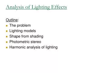
Analysis of Lighting Effects Outline: • The problem • Lighting models • Shape from shading • Photometric stereo • Harmonic analysis of lighting
Applications Modeling the effect of lighting can be used for • Recognition – particularly face recognition • Shape reconstruction • Motion estimation • Re-rendering • …
Lighting is Complex • Lighting can come from any direction and at any strength • Infinite degree of freedom
Issues in Lighting • Single light source (point, extended) vs. multiple light sources • Far light vs. near light • Matt surfaces vs. specular surfaces • Cast shadows • Inter-reflections
Lighting • From a source – travels in straight lines • Energy decreases with r2 (r – distance from source) • When light rays reach an object • Part of the energy is absorbed • Part is reflected (possibly different amounts in different directions) • Part may continue traveling through the object, if object is transparent / translucent
Specular Reflectance • When a surface is smooth light reflects in the opposite direction of the surface normal
Specular Reflectance • When a surface is slightly rough the reflected light will fall off around the specular direction
Lambertian Reflectance • When the surface is very rough light may be reflected equally in all directions
Lambertian Reflectance • When the surface is very rough light may be reflected equally in all directions
Lambert Law q or
BRDF • A general description of how opaque objects reflect light is given by the Bidirectional Reflectance Distribution Function (BRDF) • BRDF specifies for a unit of incoming light in a direction (θi,Φi) how much light will be reflected in a direction (θe,Φe) . BRDF is a function of 4 variables f(θi,Φi;θe,Φe). • (0,0) denotes the direction of the surface normal. • Most surfaces are isotropic, i.e., reflectance in any direction depends on the relative direction with respect to the incoming direction (leaving 3 parameters)
Why BRDF is Needed? Light from front Light from back
Most Existing Algorithms • Assume a single, distant point source • All normals visible to the source (θ<90°) • Plus, maybe, ambient light (constant lighting from all directions)
Shape from Shading • Input: a single image • Output: 3D shape • Problem is ill-posed, many different shapes can give rise to same image • Common assumptions: • Lighting is known • Reflectance properties are completely known – For Lambertian surfaces albedo is known (usually uniform) • First solutions: Horn, 1977
convex concave
convex concave
Lambertian Shape from Shading (SFS) • Image irradiance equation • Image intensity depends on surface orientation • It also depends on lighting and albedo, but in SFS those assumed to be known
Surface Normal • A surface z(x,y) • A point on the surface: (x,y,z(x,y))T • Tangent directions tx=(1,0,p)T, ty=(0,1,q)T with p=zx, q=zy
Lambertian SFS • We obtain • Proportionality – because albedo is known up to scale • For each point one differential equation in two unknowns, p and q • But both come from an integrable surface z(x,y) • Thus, py= qx (zxy=zyx). • Therefore, one differential equation in one unknowns (Horn, 1977)
SFS with Fast Marching • Suppose lighting coincides with viewing direction l=(0,0,1)T, then • Therefore • For general l we can rotate the camera
Distance Transform • is called Eikonal equation • Consider d(x) s.t. |dx|=1 • Assume x0=0 d x x0
Distance Transform • is called Eikonal equation • Consider d(x) s.t. |dx|=1 • Assume both x0=0 and x1=0 • Minimum at every point (shortest distance) d x x1 x0
SFS with Fast Marching • - Some places are more difficult to walk than others • Solution to Eikonal equations –using a variation of Dijkstra’s algorithm • Initial condition: we need to know z at extrema • Starting from lowest points, we propagate a wave front, where we gradually compute new values of z from old ones (Kimmel and Sethian, 2001)
Photometric Stereo (Woodham 1980) • Fewer assumptions are needed if we have several images of the same object under different lightings • In this case we can solve for both lighting, albedo, and shape • This can be done by Factorization • Recall that • Ignore the case θ>90°
Photometric Stereo - Factorization (Hayakawa, 1994) Goal: given M, find L and S What should rank(M) be?
Photometric Stereo - Factorization • Use SVD to find a rank 3 approximation • Define • So • Factorization is not unique, since , A invertible To reduce ambiguity we impose integrability
Reducing Ambiguity (Belhumeur, Kriegman, Yuille, 1999) • Assume • We want to enforce integrability • Notice that • Denote by the three rows of A, then • From which we obtain
Reducing Ambiguity • Transforming a surface linearly maintains integrability • It can be shown that this is the only transformation that maintains integrability • Such transformations are called “generalized bas relief transformations” (GBR) • Thus, by imposing integrability the surface is reconstructed up to GBR
Summary • Lighting effects are complex • Algorithms for SFS and photometric stereo for Lambertian object illuminated by a single light source • Harmonic analysis extends this to multiple light sources • Handling specularities, shadows, and inter-reflections is difficult