Download
1 / 17
170 likes | 226 Views
Learn about normal and Poisson distributions, statistical tests, errors, and contour plots, crucial for data analysis. Explore how to handle low-count regimes using C-statistic.

E N D
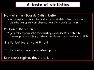
A taste of statistics • Normal error (Gaussian) distribution most important in statistical analysis of data, describes the distribution of random observations for many experiments • Poisson distribution generally appropriate for counting experiments related to random processes (e.g., radioactive decay of elementary particles) • Statistical tests: 2 and F-test • Statistical errors and contour plots • Low-count regime: the C-statistic
The Gaussian (normal error) distribution Casual errors are above and below the “true” (most “common”) value bell-shape distribution if systematic errors are negligible σ=standard deviation of the function μ=mean FWHM Г=half-width at half maximum=1.17σ
Gaussian probability function function centered on 0 function centered on μ normalization factor, so that ∫f(x) dx=1
Probability σ σ
The Poissoin distribution Describes experimental results where events are counted and the uncertainty is not related to the measurement but reflects the intrinsically casual behavior of the process (e.g., radioactive decay of particles, X-ray photons, etc.) μ>0: main parameter of the Poisson distribution ν=observed number of events in a time interval (frequency of events) average number of events μ=average number of expected events if the experiment is repeated many times
expectation value of the square of the deviations the Poisson distribution with average counts=μ has standard deviation √μ μ» : the Poisson distribution is approximated by the Gaussian distribution
Statistical tests: 2 Test to compare the observed distribution of the results with that expected Ok=observed values Ek=expected values K=number of intervals the observed and expected distributions are similar
Degrees of freedom Degrees of freedom (d.o.f.)=number of observed data – number of parameters computed from the data and used in the calculation d.o.f.=n-c where n=number of data (e.g., spectral bins) c=number of parameters which must be computed from the data to obtain the expected Ek X-ray spectral fits d.o.f.=number of spectral data points – number of free parameters
d.o.f.=channels (PHA bins) – free parameters
F-test If two statistics following the 2 distribution have been determined, the ratio of the reduced chi-squares is distributed according to the F distribution with k=number of additional terms (parameters) Example: improvement to a spectral fit due to the assumption of a different model, with possibly additional terms see the F-test tables for the corresponding probabilities (specific command in XSPEC)
An application of the F-test low F value likely low significance
Errors within XSPEC: the contour plots contour plots:show the statistical uncertainties related to two parameters 99% CONFIDENCE INTERVALSConfidence sigma (Delta)chi2 68.3% 1.0 1.00 90.0% 1.6 2.71 95.5% 2.0 4.00 99.0% 2.6 6.63 99.7% 3.0 9.00 see Avni (1976) 68% 90%
Low-counting statistic regime The fit statistic routinely used is referred to as the 2statistic where Si = src observation counts in the I={1,…,N} data bins with exposure tS, Bi = background counts with exposure tB and mi = model predicted count rate; (S)2 and (B)2 = variance on the src and background counts, typically estimated by Si and Bi BUT the 2statistic fails in low-counting regime (few counts in each data bin)
Possible solution: to rebin the data so that each bin contains • a large enough number of counts • BUT • Loss of information and dependence upon the rebinning method adopted • Viable solution: to modify S so that it performs better in • low-count regime • Estimate the variance for a given data bin by the average counts from surrounding bins (Churazov et al. 1996) BUT need for Monte-Carlo simulations to support the result
Spectrum fitted using the C-stat and then rebinned just for presentation purposes The Cash statistic Construct a maximum-likelihood estimator based on the Poisson distribution of the detected counts (Cash 1979; Wachter et al. 1979) in presence of background counts implemented into XSPEC