Part IV Data Path and Control
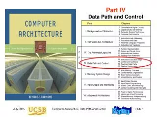
Part IV Data Path and Control. IV Data Path and Control. Design a simple computer (MicroMIPS) to learn about: Data path – part of the CPU where data signals flow Control unit – guides data signals through data path Pipelining – a way of achieving greater performance.

Part IV Data Path and Control
E N D
Presentation Transcript
Part IVData Path and Control Computer Architecture, Data Path and Control
IV Data Path and Control • Design a simple computer (MicroMIPS) to learn about: • Data path – part of the CPU where data signals flow • Control unit – guides data signals through data path • Pipelining – a way of achieving greater performance Computer Architecture, Data Path and Control
15 Pipelined Data Paths • Pipelining is now used in even the simplest of processors • Same principles as assembly lines in manufacturing • Unlike in assembly lines, instructions not independent Computer Architecture, Data Path and Control
Single-Cycle Data Path of Chapter 13 Clock rate = 125 MHz CPI = 1 (125 MIPS) Fig. 13.3 Key elements of the single-cycle MicroMIPS data path. Computer Architecture, Data Path and Control
Multicycle Data Path of Chapter 14 Clock rate = 500 MHz CPI4 (125MIPS) Fig. 14.3 Key elements of the multicycle MicroMIPS data path. Computer Architecture, Data Path and Control
Pipelined: Clock rate = 500 MHz CPI 1 Single-cycle: Clock rate = 125 MHz CPI = 1 Multicycle: Clock rate = 500 MHz CPI4 Getting the Best of Both Worlds Computer Architecture, Data Path and Control
15.1 Pipelining Concepts Strategies for improving performance 1 – Use multiple independent data paths accepting several instructions that are read out at once: multiple-instruction-issue or superscalar 2 – Overlap execution of several instructions, starting the next instruction before the previous one has run to completion: (super)pipelined Fig. 15.1 Pipelining in the student registration process. Computer Architecture, Data Path and Control
Pipelined Instruction Execution Fig. 15.2 Pipelining in the MicroMIPS instruction execution process. Computer Architecture, Data Path and Control
Alternate Representations of a Pipeline Except for start-up and drainage overheads, a pipeline can execute one instruction per clock tick; IPS is dictated by the clock frequency Fig. 15.3 Two abstract graphical representations of a 5-stage pipeline executing 7 tasks (instructions). Computer Architecture, Data Path and Control
Pipelining Example in a Photocopier Example 15.1 A photocopier with an x-sheet document feeder copies the first sheet in 4 s and each subsequent sheet in 1 s. The copier’s paper path is a 4-stage pipeline with each stage having a latency of 1s. The first sheet goes through all 4 pipeline stages and emerges after 4 s. Each subsequent sheet emerges 1s after the previous sheet. How does the throughput of this photocopier varies with x, assuming that loading the document feeder and removing the copies takes 15 s. Solution Each batch of x sheets is copied in 15 + 4 + (x – 1) = 18 + x seconds. A nonpipelined copier would require 4x seconds to copy x sheets. For x > 6, the pipelined version has a performance edge. When x = 50, the pipelining speedup is (4 50) / (18 + 50) = 2.94. Computer Architecture, Data Path and Control
15.2 Pipeline Stalls or Bubbles First type of data dependency Fig. 15.4 Read-after-write data dependency and its possible resolution through data forwarding . Computer Architecture, Data Path and Control
Second Type of Data Dependency Fig. 15.5 Read-after-load data dependency and its possible resolution through bubble insertion and data forwarding. Computer Architecture, Data Path and Control
Control Dependency in a Pipeline Fig. 15.6 Control dependency due to conditional branch. Computer Architecture, Data Path and Control
15.3 Pipeline Timing and Performance Fig. 15.7 Pipelined form of a function unit with latching overhead. Computer Architecture, Data Path and Control
t t/q + or q 1 + q/t Throughput Increase in a q-Stage Pipeline Fig. 15.8 Throughput improvement due to pipelining as a function of the number of pipeline stages for different pipelining overheads. Computer Architecture, Data Path and Control
q (1 + q/t)(1 + b) Pipeline speedup = Pipeline Throughput with Dependencies Assume that one bubble must be inserted due to read-after-load dependency and after a branch when its delay slot cannot be filled. Let be the fraction of all instructions that are followed by a bubble. R-type 44% Load 24% Store 12% Branch 18% Jump 2% Example 15.3 Calculate the effective CPI for MicroMIPS, assuming that a quarter of branch and load instructions are followed by bubbles. Solution Fraction of bubbles b = 0.25(0.24 + 0.18) = 0.105 CPI = 1 + b = 1.105 (which is very close to the ideal value of 1) Computer Architecture, Data Path and Control
15.4 Pipelined Data Path Design Fig. 15.9 Key elements of the pipelined MicroMIPS data path. Computer Architecture, Data Path and Control
15.5 Pipelined Control Fig. 15.10 Pipelined control signals. Computer Architecture, Data Path and Control
15.6 Optimal Pipelining MicroMIPS pipeline with more than four-fold improvement Fig. 15.11 Higher-throughput pipelined data path for MicroMIPS and the execution of consecutive instructions in it . Computer Architecture, Data Path and Control
Optimal Number of Pipeline Stages Assumptions: Pipeline sliced into q stages Stage overhead is t q/2 bubbles per branch (decision made midway) Fraction b of all instructions are taken branches Fig. 15.7 Pipelined form of a function unit with latching overhead. Derivation of qopt Average CPI = 1 + bq / 2 Throughput = Clock rate / CPI = [(t/q + t)(1 + bq / 2)]–1/2 Differentiate throughput expression with respect to q and equate with 0 qopt = [2(t/t) / b)]1/2 Computer Architecture, Data Path and Control

