Download

1 / 66
660 likes | 796 Views
Assessing complexity of short-term heart period variability through entropy-based approaches. Alberto Porta. Department of Biomedical Sciences for Health Galeazzi Orthopedic Institute University of Milan Milan, Italy. Introduction.

E N D
Assessing complexity of short-term heart period variability through entropy-based approaches Alberto Porta Department of Biomedical Sciences for Health Galeazzi Orthopedic Institute University of Milan Milan, Italy
Introduction Several physiological control systems are responsible to the changes of heart period on a beat-to-beat basis. These control mechanisms interact each other and might even compete The visible result is the richness of dynamics of heart period when observed on a beat-to-beat basis (i.e. the complexity of heart period series) Some observations suggest that measuring complexity of heart period might provide useful clinical information (e.g. it decreases with age and disease)
Primary aim To monitor complexity of heart period dynamics via entropy-based approaches
Definition of heart period variability series ECG RR=RR(i), i=1,…,N
Short-term heart period variability Heart period series exhibits non random fluctuations when observed over a temporal scale of few minutes These fluctuations are referred to as short-term heart period variability
Autonomic regulation of heart period Heart rate variability is under control of the autonomic nervous system Saul JP et al, Am J Physiol, 256:H153-H161, 1989
Power in the LF band LF/HF = Power in the HF band Assessing autonomic balance via spectral analysis Monitoring heart rate variability has become very popular to assess balancing between parasympathetic and sympathetic regulation LF HF LF band: 0.04f0.15 Hz HF band: 0.15<f0.5 Hz Akselrod S et al, Science, 213:220-223, 1981 Malliani A et al, Circulation, 84:482-492, 1991 Task Force, Circulation 93:1043-1065, 1996
Drawbacks of the evaluation of the autonomic balance based on spectral analysis • LF/HF index is based on a linear analysis • LF/HF index depends on the definition of the limits of the • frequency bands • 3) The numerator and denominator of the LF/HF index are not • independent • 4) LF/HF index loses his meaning when respiration drops in the • LF band
Secondary aim Are entropy-based complexity indexes helpful to infer the state of the autonomic nervous system controlling heart rate?
Short-term heart period variability complexity and autonomic nervous system Tulppo MP et al, Am J Physiol, 280:H1081-H1087, 2001
Short-term heart period variability complexity and autonomic nervous system Porta A et al, IEEE Trans Biomed Eng, 54:94-106, 2007
Aims • To verify whether complexity indexes based on entropy rates can • track the gradual increase of sympathetic modulation (and the • concomitant decrease of vagal one) produced by graded head-up • tilt test • To compare well-established estimates of entropy rates on the • same experimental protocol • 3) To understand whether normalization of entropy rate with respect • to an index of static complexity may bring additional information
Pattern definition Given the series RR = RR(i), i=1,...,N Pattern: RRL(i) = (RR(i),RR(i-1),...,RR(i-L+1)) A pattern is a point in a L-dimensional embedding space With L=3 RR(i-1) RRL=3(i) RR(i) RR(i-2)
Shannon entropy (SE) and conditional entropy (CE) Shannon entropy (SE) SE(L) = -Sp(RRL(i)).log(p(RRL(i))) Conditional entropy (CE) CE(L) = SE(L)-SE(L-1)
Functions playing a role equivalent to the conditional entropy 1) Approximate entropy (ApEn) 2) Sample entropy (SampEn) 3) Corrected conditional entropy (CCE) Pincus SM, Chaos, 5:110-117, 1995 Richman JS and Moorman JR, Am J Physiol, 278:H2039-H2049, 2000 Porta A et al , Biol Cybern, 78:71-78, 1998
RR(i-1) RRL(j) r RRL(i) RR(i) RR(i-2) Pattern similarity within a tolerance r With L=3 RRL(j) is similar to RRL(i) within a tolerance r if they RRL(j) is closer than r to RRL(i) According to the Euclidean norm, RRL(j) is similar to RRL(i) if RRL(j) lies in a hyper-sphere of radius r centered in RRL(i)
N-L+1 1 PS(L,r)= - Slog(Ci(L,r)) N-L+1 i=1 Ni(L,r) N-L+1 Approximate entropy (ApEn) where Ci(L,r) = Ni(L,r) = number of points (i.e. patterns) similar to RRL(i) within a tolerance r ApEn(L,r) = PS(L,r) - PS(L-1,r) Pincus SM, Chaos, 5:110-117, 1995
RR(i-1) r RRL(i) RR(i) RR(i-2) Self-matching Self-matching is a consequence of the trivial observation that RRL(j) is always at distance smaller than r from RRL(i) when i=j With L=3 Self-matching occurs when the unique pattern in the hyper-sphere of radius r centered around RRL(i) is RRL(i) RRL(i) is a “self-match” if Ni(L,r)=1
N-L+1 1 PS(L,r)= - Slog(Ci(L,r)) N-L+1 i=1 ≤Ci(L,r) ≤1 1 N-L+1 Self-matching and approximate entropy When calculating self-matching is allowed log(0) is prevented
Bias of the approximate entropy Two factors produce the important bias of ApEn 1) due to the spreading of the dynamics in the phase space Ni(L,r)≤Ni(L-1,r) 2) due to self-matching Ni(L,r)1 Ni(L,r) 1 while increasing L
Bias of the approximate entropy Since Ni(L,r) 1 while increasing L PS(L,r) PS(L-1,r) ApEn(L,r) = PS(L,r) - PS(L-1,r) 0 thus producing a bias toward regularity
Approximate entropy over a realization of a Gaussian white noise r=0.2.SD N=300 ApEn(L=2,r,N) 76.5% The high percentage of “self-matches” even at small L makes mandatory their optimal management
N-L+1 - Slog ApEn(L,r)=PS(L,r) - PS(L-1,r) = i=1 1 Ni(L,r) N-L+1 Ni(L-1,r) Correction: When Ni(L,r)=1 or Ni(L-1,r)=1, then is set to Ni(L,r) 1 Ni(L-1,r) N-L+1 Correction of the approximate entropy: the corrected ApEn (CApEn) Porta A et al, J Appl Physiol, 103:1143-1149, 2007
Ni(L,r) N-L+1 Sample entropy (SampEn) N-L+1 1 RM(L,r) = - log( SCi(L,r)) N-L+1 i=1 where Ci(L,r) = Ni(L,r) = number of points (i.e. patterns) that can be found at distance smaller than r from RRL(i) SampEn(L,r) = RM(L,r) - RM(L-1,r) Richman JS and Moorman JR, Am J Physiol, 278:H2039-H2049, 2000
N-L+1 SNi(L,r) - log i=1 SampEn(L,r)=RM(L,r) - RM(L-1,r) = N-L+1 SNi(L-1,r) i=1 Self-matching and sample entropy When calculating SampEn(L,r) “self-matches” are excluded Ni(L,r) and Ni(L-1,r) can be 0
Toward an approximation of Shannon entropy and conditional entropy: uniform quantization max(RR)-min(RR) q=6 with ε = q RR(i), i=1,...,N with RR(i) R ε RRq(i), i=1,...,N with RRq(i) I 0RRq(i)q-1
Estimation of Shannon entropy and conditional entropy Given the quantized series RRq = RRq(i), i=1,...,N and built the series of quantized patterns RRLq = RRLq(i), i=L,...,N with RRLq(i) = (RRq(i),RRq(i-1),...,RRq(i-L+1)) Shannon entropy (SE) SE(L,q) = -Sp(RRLq(i)).log(p(RRLq(i))) Conditional entropy (CE) CE(L,q) = SE(L,q)-SE(L-1,q)
Definition of “single” patterns Let’s define as “single” the quantized pattern RRLq(i) such that it is alone in an hypercube of the partition of the phase space imposed by uniform quantization
1 1 1 1 - log( ) ≈ - log( ) N-L+1 N-L+1 N N Bias of the estimate of the conditional entropy The contribution of each “single” pattern to Shannon entropy is Since it N>>L, it is constant with L and, thus, its contribution to the conditional entropy is 0 “Single” patterns do not contribute to CE
Bias of the estimate of the conditional entropy and single patterns Since the percentage of “single” patterns increases as a function of L, the conditional entropy decreases to 0
CCE(L,q) CE(L,q) SE(L=1,q) . perc(L) Corrected conditional entropy (CCE) CCE(L,q) = CE(L,q) + SE(L=1,q).fraction(L) with 0perc(L)1 Porta A et al , Biol Cybern, 78:71-78, 1998
Experimental protocol 17 healthy young humans (age from 21 to 54, median=28) We recorded ECG (lead II) and respiration (thoracic belt) at 1 kHz during head-up tilt (T) Each T session (10 min) was always preceded by a session (7 min) at rest (R) and followed by a recovery period (3 min) Table angles were randomly chosen within the set {15,30,45,60,75,90}
Setting for calculation of the complexity indexes • Approximate entropy, ApEn(L,r,N) and Corrected • Approximate entropy, CApEn(L,r,N) • L-1=2; r=0.2.SD; N=250 • 2) Sample entropy, SampEn(L,r,N) • L-1=2; r=0.2.SD; N=250 • 3) Corrected conditional entropy, CCE(L,q,N) • L=Lmin; q=6; N=250 CIPS CCIPS CIRM CIP
CIPS NCIPS = CIPS CCIPS CIRM CIP PS(L=1,r) CCIPS NCCIPS = PS(L=1,r) CIRM NCIRM = RM(L=1,r) CIP NCIP = SE(L=1,) Normalized complexity indexes
Entropy-based complexity indexes during graded head-up tilt Values are expressed as median (first quartile – third quartile). CI = complexity index; NCI = normalized CI; CCI = corrected CI; NCCI = normalized CCI; subscripts PS, RM, P (Pincus, Richman and Moorman, and Porta) indicate the name of the authors who proposed the index. The symbol # indicates a significant difference vs R with p<0.05. Porta A et al, J Appl Physiol, 103:1143-1149, 2007
Global linear regression (GLR) analysis of entropy-based complexity indexes on tilt angles Yes/No = presence/absence of a significant global linear correlation. Porta A et al, J Appl Physiol, 103:1143-1149, 2007
Correlation coefficient of global linear regression (GLR) of entropy-based complexity indexes on tilt angles rGLR = global correlation coefficient. Porta A et al, J Appl Physiol, 103:1143-1149, 2007
Individual trends of entropy-based complexity indexes based on ApEn Porta A et al, J Appl Physiol, 103:1143-1149, 2007
Individual trends of entropy-based complexity indexes based on CApEn Porta A et al, J Appl Physiol, 103:1143-1149, 2007
Individual trends of entropy-based complexity indexes based on SampEn Porta A et al, J Appl Physiol, 103:1143-1149, 2007
Individual trends of entropy-based complexity indexes based on CCE Porta A et al, J Appl Physiol, 103:1143-1149, 2007
Individual linear regression (ILR) analysis of entropy-based complexity indexes on tilt angles ILR% = fraction of subjects with significant individual linear correlation; = quantization levels. Porta A et al, J Appl Physiol, 103:1143-1149, 2007
Conclusions Approximate entropy was unable to follow the progressive decrease of complexity of short-term heart period variability during graded head-up tilt Entropy-based indexes of complexity, when computed appropriately by correcting the bias that arises from their evaluation over short sequences, progressively decrease as a function of tilt table inclination These indexes appear to be suitable to quantify the balance between parasympathetic and sympathetic regulation
Effects of pharmacological challenges on entropy-based complexity of short-term heart period variability