Download
1 / 31
321 likes | 462 Views
The role of relative accessibility in urban built environment. Slavomír Ondoš , Shanaka Herath. Overview. Introduction: location in a polycentric urban context Methods: space syntax and spatial econometrics Results: distance to CBD vs. network integration Conclusions. Introduction.

E N D
The role of relativeaccessibility in urbanbuilt environment SlavomírOndoš, ShanakaHerath
Overview • Introduction: location in a polycentric urban context • Methods: space syntax and spatial econometrics • Results: distance to CBD vs. network integration • Conclusions
Introduction • Location of real estate projects is one of the most important decisions made at the beginning of any development process. • Once a property is constructed, it is attached to the place throughout the whole life cycle and it keeps affecting location of other investments in the neighborhood. • Relative accessibility of the components integrated in the urban structures may explain how potential spatial interactions between them shape the urban pattern.
Introduction • The standard urban model is monocentric. • The principal variable causing variations in constant-quality house prices within a metropolitan area is land price. A typical land rental equation therefore includes distance from the center, agricultural land rental, a conversion parameter that depends on transport cost per distance and community income. • Firms and households are willing to bid more for land that is closer to the center because transport costs will be lower.
Introduction • The controversies between the monocentric and the polycentric nature of cities and their implications for estimation are discussed in the literature. • Dubin (1992), for instance, states that non-CBD peaks in the rent gradient cause traditional means of capturing accessibility effects to give inconclusive results. • These findings direct towards a more flexible means of capturing neighborhood and accessibility effects, which allow for multiple peaks in the rent surface.
Introduction • Spatial interaction models are mathematical formulations used to analyze and forecast spatial interaction patterns. • They are concerned not about the absolute but the relative location. • In the local level, locations are different in a multitude of ways (access to shopping, job opportunities, museums and theatres, rural life-styles, wilderness opportunities, etc). The spatial interaction models measure explicitly such relative location concepts.
Introduction • Space syntax is a collection of topological relative location, accessibility and spatial integration measures (discarding metrics). • First applications have studied the correlation between integration and distribution of pedestrian movements constructed to help architects simulate the likely social effects of their design (Hillier et al. 1983, Hillier and Hanson 1984, Hillier 1988 and 1996). • Subsequently it was used in urban studies and regional science (Brown 1999, Kim and Sohn 2002, Enström and Netzell 2008).
Introduction • We examine the relationship between relative accessibility and built environment density in Bratislava, Slovak Republic, with its emerging post-socialist real estate market between the years 1991 and 2006. • Question 1: The better integrated locations are more attractive subject to competition resulting in a higher built environment density. • Question 2: The transition period documents a process of density gradient restoration driven significantly by the relative accessibility.
Central Bratislava, 1991in 100 m raster 0.00 - 0.50 0.50 – 0.15 0.15 – 0.30 0.30 – 0.60 0.60 – 100.00
Central Bratislava, 2006in 100 m raster 0.00 - 0.50 0.50 – 0.15 0.15 – 0.30 0.30 – 0.60 0.60 – 100.00
Methods • Approaching directly our research questions we construct three regression models explaining built environment density measured on urban topography in both time horizons as well as the difference during the 15 years between D1991 = a + bx + e D2006 = a + bx + e DD1991-2006 = a + bDx + e • Two explanatory variables will be considered
Methods • Distance DIS1991(2006) captures the effect from Euclidean distance between the cell and the gravity point having its coordinates as mean values from total cellular space. The weights used are D1991 and D2006. • Integration INT1991(2006) quantifies average global integration resulting from the position of a cell in the street network transformed into an axial system used by the space syntax methodology.
Methods • Mean depth mDi = Di / (L-1) indicates how close is an average axial line to all other axial lines in the system if dij is topological distance Di = SL-1j=1, j≠idij • Relative asymmetry in the empirical system is then compared with the diamond-shaped street network system resulting in the standardized value of integration (Enström and Netzell 2008) RAi = 2(mDi – 1) / (L–2) INT = RAD/RAi
Central Bratislava, 2006street network integration 0.49 - 0.76 0.76 – 0.90 0.90 – 1.03 1.03 – 1.17 1.17 – 1.45
Central Bratislava, 2006street network integration 0.49 - 0.76 0.76 – 0.90 0.90 – 1.03 1.03 – 1.17 1.17 – 1.45
Methods • Since the three constructed models will necessarily incorporate spatial effects (from vector → raster data transformation, spatial interaction within the urban system), we must provide regression diagnostics and diagnostics for spatial dependence. • Two alternative estimations considered will be the spatial lag model and the spatial error model D = a + rWD + bx + e D = a + bx + e, e = lWe + z
Model selection DLL = 32,000, Ddf = 1 (> 3,841, a = 0,05) DLL = 30,000, Ddf = 1 (> 3,841, a = 0,05) DLL = 2,000, Ddf = 1 (< 3,841, a = 0,05) DLL = 23,826, Ddf = 1 (> 3,841, a = 0,05)
Conclusions • Question 1: The better integrated locations are more attractive subject to competition resulting in higher built environment density. • The more intensively urbanized locations are those better integrated within the street network and these are also closer to the gravity point (negative effect from distance). • This regularity is found in both 1991 and 2006 with an identical effect from distance and slightly decreasing effect from integration.
Conclusions • Question 2: The transition period documents a process of density gradient restoration driven significantly by relative accessibility. • The locations with improved integration and approaching the flowing center have been significantly more urbanized during the 15 years than those which became less integrated. • The negative effect from distance to gravity point is found significant only in presence of integration explanatory variable. The model attempting to explain it by distance alone has a serious specification problem.
Conclusions • Question 2: The transition period documents a process of density gradient restoration driven significantly by relative accessibility. • Significantly more urbanized during the same period were those locations with lower integration value, closer to the center and less urbanized in 1991. • The negative effects from distance to gravity point, integration and urbanization level in 1991 are found significant in all three cases correctly specified as spatial error models.
Conclusions • Parameter values identifying spatial effects in both alternative models r and l are positive and significant without any exception. • Locations tend to be more intensively urbanized if they have more urbanized neighborhood in compare to those with less intensively urbanized neighborhood. • The models explaining density by distance alone are driven towards the spatial error alternative. The models explaining density by integration are driven towards theoretically superior spatial lag alternative (except the 4th alternative).
Forschungsinstitut für Raum- und Immobilienwirtschaft Research Institute for Spatial and Real Estate Economics Nordbergstraße 15, 1090 Vienna, Austria MGR. SLAVOMÍR ONDOŠ T +43-1-313 36-5764 F +43-1-313 36-705 slavomir.ondos@wu-wien.ac.at www.wu.ac.at/immobilienwirtschaft