Download
1 / 1
10 likes | 141 Views
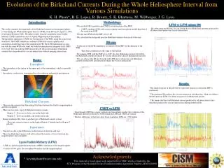
Evolution of the Birkeland Currents During the Whole Heliosphere Interval from Various Simulations. K. H. Pham*, R. E. Lopez, R. Bruntz, S. K. Bhattarai, M. Wiltberger, J. G. Lyon. Introduction

E N D
Evolution of the Birkeland Currents During the Whole Heliosphere Interval from Various Simulations K. H. Pham*, R. E. Lopez, R. Bruntz, S. K. Bhattarai, M. Wiltberger, J. G. Lyon Introduction This study examines the magnitude of the Birkeland currents in the magnetospheric system during the Whole Heliosphere Interval (WHI), from March 20-April 16, 2008 (Carrington Rotation 2068). We utilize results from the standalone Lyon-Fedder-Mobarry (LFM) simulations and a Coupled Magnetosphere-Ionosphere-Thermosphere simulation (CMIT) for the duration of the WHI, using the actual solar wind data. The CMIT simulation combines LFM with a more sophisticated ionospheric model than that of the standalone LFM. The LFM simulation was also run with the same WHI solar wind, but with the interplanetary magnetic field (IMF) set to 0 nT. The run with the IMF turned off will tell us the amount of Birkeland currents that are produced by viscous interactions without merging interactions. • Methodology • We ran the LFM simulation and CMIT for the duration of the WHI • CMIT combines LFM with a more sophisticated ionospheric model than that of the standalone LFM • We also ran LFM with the IMF set to 0 nT • We calculated the integrated positive Birkeland currents from each of the runs • LFM vs LFM minus B0 • By subtracting the B0 run, we can obtain the total Birkeland currents produced by all interactions minus the viscous interactions • B0 run • In this run of the LFM simulation, we turned off the IMF for the duration of the WHI • The other conditions are the same as the full run • By running LFM with the IMF set to 0 nT, the only Birkeland currents left will be the Birkeland currents produced by viscous interactions and not merging interactions • We can subtract the B0 run from the full LFM run to obtain the total Birkeland currents produced by all interactions minus the viscous interactions • Basics Ionosphere • The ionosphere is the region in the upper part of the atmosphere, which is partially ionized • Ionospheric conductivity is produced by solar radiation and particle precipitation • Birkeland Currents • These are the currents that flow along field lines between the Earth’s magnetosphere and the ionosphere • There are two basic types of Birkeland current systems: • Region 1 ~ flows in on dawn, out on the dusk side • Region 2 ~ flows in on dusk, out on the dawn side • During northward Bz, there is another type of Birkeland current system • This type current system is in the highest Region 1 latitude but has Region 2 polarity • Importance • Currents are due to the differences in the motion of electrons and ions • Therefore Birkeland currents will tell us about the transfer of stress between the magnetosphere and ionosphere • Results • The shaded regions in the plot below represents regions in which the IMF is northward • The northward Bz reduces the viscous interaction and therefore, when we subtract the B0 run from LFM, we obtain a negative total Birkeland current • This means that the total Birkeland current produced by all interactions is less than that produced by viscous interactions during northward Bz • CMIT vs LFM • Even though CMIT has a more sophisticated ionospheric model, the evolution of the Birkeland currents produced by both standalone LFM and CMIT are similar • The key difference is that the values from standalone LFM are ~50% higher • Lyon-Fedder-Mobarry (LFM) • LFM is a global magnetohydrodynamic (MHD) simulation of the magnetosphere • Consists of two parts, the ionosphere boundary and the magnetosphere Acknowledgments This material is based upon work supported by CISM, which is funded by the STC Program of the National Science Foundation under Agreement Number ATM-0120950 * kevinhpham@mavs.uta.edu