Download
1 / 46
460 likes | 607 Views
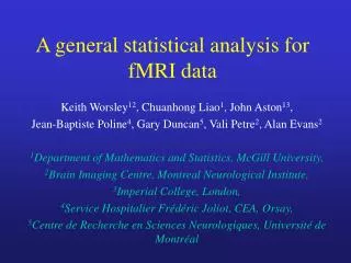
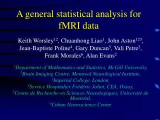
A general statistical analysis for fMRI data. Keith Worsley 12 , Chuanhong Liao 1 , John Aston 123 , Jean-Baptiste Poline 4 , Gary Duncan 5 , Vali Petre 2 , Frank Morales 6 , Alan Evans 2 1 Department of Mathematics and Statistics, McGill University,

E N D
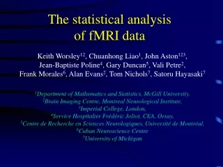
A general statistical analysis for fMRI data Keith Worsley12, Chuanhong Liao1, John Aston123, Jean-Baptiste Poline4, Gary Duncan5, Vali Petre2, Frank Morales6, Alan Evans2 1Department of Mathematics and Statistics, McGill University, 2Brain Imaging Centre, Montreal Neurological Institute, 3Imperial College, London, 4Service Hospitalier Frédéric Joliot, CEA, Orsay, 5Centre de Recherche en Sciences Neurologiques, Université de Montréal, 6Cuban Neuroscience Centre
fMRI data: 120 scans, 3 scans each of hot, rest, warm, rest, hot, rest, … (a) Highly significant correlation 960 hot fMRI data rest 940 warm 920 0 50 100 150 200 250 300 350 400 940 (b) No significant correlation hot fMRI data 920 rest warm 900 0 50 100 150 200 250 300 350 400 850 fMRI data 840 (c) Drift 830 0 50 100 150 200 250 300 350 400 Time, t (seconds) Z = (effect hot – warm) / S.d. ~ N(0,1) if no effect
FMRISTAT: Simple, general, valid, robust, fast analysis of fMRI data • Linear model: • ? ? • Yt = (stimulust * HRF) b + driftt c + errort • AR(p) errors: • ? ? ? • errort = a1 errort-1 + … + ap errort-p + s WNt unknown parameters
(a) Stimulus, s(t): alternating hot and warm stimuli on forearm, separated by rest (9 seconds each). 2 warm warm hot hot 1 0 -1 0 50 100 150 200 250 300 350 400 (b) Hemodynamic response function, h(t): difference of two gamma densities (Glover, 1999) 0.4 0.2 0 -0.2 0 50 100 150 200 250 300 350 400 2 1 0 -1 0 50 100 150 200 250 300 350 400 FMRIDESIGN example: Pain perception (c) Response, x(t): sampled at the slice acquisition times every 3 seconds Time, t (seconds)
FMRILM step 1: estimate temporal correlation ? AR(1) model: errort = a1errort-1 + s WNt • Fit the linear model using least squares. • errort = Yt – fitted Yt â1 = Correlation ( errort , errort-1) • Estimating errort’schanges their correlation structure slightly, so â1 is slightly biased. • Bias correction is very quick and effective: Raw autocorrelation Smoothed 15mm Bias corrected â1 ~ -0.05 ~ 0
T > 4.90 (P < 0.05, corrected) FMRILM step 2: refit the linear model Pre-whiten: Yt* = Yt – â1 Yt-1, then fit using least squares: Effect: hot – warm Sd of effect T statistic = Effect / Sd
Higher order AR model? Try AR(4): â1 â2 ~ 0 â3 â4 ~ 0 ~ 0 AR(1) seems to be adequate
But ignoring correlation … biases T up ~12% more false positives … has no effect on the T statistics: AR(1) AR(2) AR(4)
Results from 4 runs on the same subject Run 1 Run 2 Run 3 Run 4 Effect Ei Sd Si T stat Ei / Si
MULTISTAT combines effects from different runs/sessions/subjects: • Ei = effect for run/session/subject i • Si = standard error of effect • Mixed effects model: Ei = covariatesi c + Si WNiF + WNiR }from FMRILM ? ? Usually 1, but could add group, treatment, age, sex, ... ‘Fixed effects’ error, due to variability within the same run Random effect, due to variability from run to run
REML estimation of the mixed effects model using the EM algorithm • Slow to converge (10 iterations by default). • Stable (maintains estimate 2 > 0 ), but • 2 biased if 2 (random effect) is small, so: • Re-parametrise the variance model: Var(Ei) = Si2 + 2 = (Si2 –minj Sj2) + (2 +minj Sj2) = Si*2 + *2 • 2 = *2 –minj Sj2 (less biased estimate) ^ ^ ? ? ^ ^
Problem: 4 runs, 3 df for random effects sd ... Run 1 Run 2 Run 3 Run 4 MULTISTAT Effect Ei … very noisy sd: Sd Si … and T>15.96 for P<0.05 (corrected): T stat Ei / Si … so no response is detected …
Solution: Spatial regularization of the sd • Basic idea: increase df by spatial smoothing (local pooling) of the sd. • Can’t smooth the random effects sd directly, - too much anatomical structure. • Instead, • random effects sd • fixed effects sd • which removes the anatomical structure before smoothing. ) sd= smooth fixed effects sd
Regularized sd (112 df) Random effects sd Fixed effects sd Fixed effects sd Over runs Over subjects Smooth 15mm ~1 ~3 ~1.6 Random effects sd (3 df) Fixed effects sd (448 df)
Effective df depends on the smoothing FWHMratio2 3/2 FWHMdata2 dfratio = dfrandom(2 + 1) 1 1 1 dfeffdfratiodffixed e.g. dfrandom = 3, dffixed = 112, FWHMdata = 6mm: FWHMratio (mm) 0 5 10 15 20 infinite dfeff 3 11 45 112 192 448 = + Random effectsFixed effects variability bias compromise!
Final result: 15mm smoothing, 112 effective df … Run 1 Run 2 Run 3 Run 4 MULTISTAT Effect Ei … less noisy sd: Sd Si … and T>4.90 for P<0.05 (corrected): T stat Ei / Si … and now we can detect a response!
Conjunction: All Ti > threshold = Min Ti > threshold ‘Minimum of Ti’ ‘Average of Ti’ For P=0.05, threshold = 1.82 For P=0.05, threshold = 4.90 Efficiency = 82%
If the conjunction is significant, does it mean that all effects > 0? • Problem: for the conjunction of 20 effects, the threshold can be negative!?!?! • Reason: significance is based on the wrong null hypothesis, namely: all effects = 0 • Correct null hypothesis is: at least one effect = 0. Unfortunately the P-value depends on the unknown > 0 effects … • If the effects are random, all effects > 0 is meaningless. The only parameter is the (single) population effect, so that the conjunction just tests if population effect > 0. • P-values now depend on the random effects sd, not the fixed effects sd. But the minimum (i.e. the conjunction) is less efficient (sensitive) than the average (the usual test).
FWHM – the local smoothness of the noise · • Used by STAT_THRESHOLD to find the P-value of local maxima and the spatial extent of clusters of voxels above a threshold. • u = normalised residuals from linear model = residuals / sd • u = vector of spatial derivatives of u • λ = |Var(u)|1/2 (mm-3) • FWHM = (4 log 2)1/2λ-1/3 (mm) (If residuals are modeled as white noise smoothed with a Gaussian kernel, this would be its FWHM). • λ and FWHM are corrected for low df and large voxel size so they are approximately unbiased. • For a search region S, the number of ‘resolution elements’ is Resels(S) = Vol(S) AvgS(FWHM-3) = Vol(S) AvgS(λ) (4 log 2)-3/2 • For local maxima in S, P_value = Resels(S) x (function of threshold). • For a cluster C, P-value depends on Resels(C) instead of Vol(C), so that clusters in smooth regions are less significant. • Need a correction for the randomness ofλ and FWHM - depends on df . • Correction is more important for small clusters C than for large search regions S. ·
FWHM (mm) over scans (448 df) FWHM (mm) over runs (3 df) 20 20 15 15 10 10 5 5 0 0 smoothed FWHM over runs smoothed (runs FWHM / scans FWHM) 20 1.5 15 10 1 5 0 0.5 …. FWHM depends on the spatial correlation between neighbours Resels=1.90 P=0.007 Resels=0.57 P=0.387
T > 4.90 (P < 0.05, corrected) T>4.86
Smooth the data before analysis? • Temporal smoothing or low-pass filtering is used by SPM’99 to validate a global AR(1) model. For our local AR(p) model, it is not necessary (but ~ harmless). • Spatial smoothing is used by SPM’99 to validate random field theory. Can be harmful for focal signals. Should fix the theory! STAT_THRESHOLD uses the better of the Bonferroni or the random field theory. • A better reason for spatial smoothing is greater detectability of extensive activation: choose the FWHM to match the activation (e.g. 10mm FWHM for 10mm activations) – or try a range of FWHM’s i.e. scale space – but thresholds are higher …
False Discovery Rate (FDR) • Benjamini and Hochberg (1995), Journal of the Royal Statistical Society • Benjamini and Yekutieli (2001), Annals of Statistics • Genovese et al. (2001), NeuroImage • FDR controls the expected proportion of false positives amongst the discoveries, whereas • Bonferroni / random field theory controls the probability of any false positives • No correction controls the proportion of false positives in the volume
Signal + Gaussian white noise P < 0.05 (uncorrected), Z > 1.64 5% of volume is false + Signal True + Noise False + FDR < 0.05, Z > 2.82 5% of discoveries is false + P < 0.05 (corrected), Z > 4.22 5% probability of any false +
Comparison of thresholds • FDR depends on the ordered P-values (not smoothness): • P1 < P2 < … < Pn. To control the FDR at a = 0.05, find • K = max {i : Pi< (i/n) a}, threshold the P-values at PK • Proportion of true + 1 0.1 0.01 0.001 0.0001 • Threshold Z 1.64 2.56 3.28 3.88 4.41 • Bonferroni thresholds the P-values at a/n: • Number of voxels 1 10 100 1000 10000 • Threshold Z 1.64 2.58 3.29 3.89 4.42 • Random field theory: resels = volume / FHHM3: • Number of resels 0 1 10 100 1000 • Threshold Z 1.64 2.82 3.46 4.09 4.65
P < 0.05 (uncorrected), Z > 1.64 5% of volume is false + FDR < 0.05, Z > 2.91 5% of discoveries is false + P < 0.05 (corrected), Z > 4.86 5% probability of any false + Which do you prefer?
0.6 0.4 0.2 0 -0.2 -0.4 -5 0 5 10 15 20 25 t (seconds) Estimating the delay of the response • Delay or latency to the peak of the HRF is approximated by a linear combination of two optimally chosen basis functions: delay basis1 basis2 HRF shift • HRF(t + shift) ~ basis1(t)w1(shift) + basis2(t)w2(shift) • Convolve bases with the stimulus, then add to the linear model
3 2 1 0 -1 -2 -3 -5 0 5 shift (seconds) • Fit linear model, estimate w1andw2 • Equate w2/w1to estimates, then solve for shift (Hensen et al., 2002) • To reduce bias when the magnitude is small, use • shift / (1 + 1/T2) • where T = w1/ Sd(w1) is the T statistic for the magnitude • Shrinks shift to 0 where there is little evidence for a response. w2 /w1 w1 w2
5 5 0 0 -5 -5 10 5 8 4 6 3 4 2 2 1 0 0 Delay of the hot stimulus (= shift + 5.4 sec) T stat for magnitude T stat for shift Delay (secs) Sd of delay (secs)
5 5 10.4 10.4 0 0 5.2 5.2 2.6 2.6 -5 -5 2.4 5.4 8.4 2.4 5.4 8.4 Reference dispersion (seconds) 10 5 10.4 10.4 8 4 6 3 5.2 5.2 4 2 2 1 2.6 2.6 0 0 2.4 5.4 8.4 2.4 5.4 8.4 Reference delay (seconds) Varying the delay and dispersion of the reference HRF T stat for magnitude T stat for shift Delay (secs) Sd of delay (secs)
T > 4.86 (P < 0.05, corrected) Delay (secs) 6.5 5 5.5 4 4.5
T > 4.86 (P < 0.05, corrected) Delay (secs) 6.5 5 5.5 4 4.5
EFFICIENCY for optimum block design Sd of hot stimulus Sd of hot-warm 0.5 0.5 20 20 0.4 0.4 15 15 Magnitude Optimum design 0.3 0.3 10 10 Optimum design 0.2 0.2 X 5 5 0.1 0.1 0 0 X 0 0 5 10 15 20 5 10 15 20 InterStimulus Interval (secs) (secs) (secs) 1 1 20 20 0.8 0.8 15 15 Delay 0.6 0.6 Optimum design X Optimum design X 10 10 0.4 0.4 5 5 0.2 0.2 (Not enough signal) (Not enough signal) 0 0 0 5 10 15 20 5 10 15 20 Stimulus Duration (secs)
EFFICIENCY for optimum event design 0.5 (Not enough signal) uniform . . . . . . . . . ____ magnitudes ……. delays random .. . ... .. . 0.45 concentrated : 0.4 0.35 0.3 Sd of effect (secs for delays) 0.25 0.2 0.15 0.1 0.05 0 5 10 15 20 Average time between events (secs)
+ + How many subjects? • Variance = sdrun2sdsess2sdsubj2 nrunnsessnsubj nsessnsubj nsubj • The largest portion of variance comes from the last stage, i.e. combining over subjects. • If you want to optimize total scanner time, take more subjects, rather than more scans per subject. • What you do at early stages doesn’t matter very much - any reasonable design will do …
Comparison • Different slice acquisition times: • Drift removal: • Temporal correlation: • Estimation of effects: • Rationale: • Random effects: • FWHM: • Map of delay: • SPM’99: • Adds a temporal derivative • Low frequency cosines (flat at the ends) • AR(1), global parameter, bias reduction not necessary • Band pass filter, then least-squares, then correction for temporal correlation • More robust, low df • No regularization, low df • Global, ~ OK for local maxima, but not clusters • No • FMRISTAT: • Shifts the model • Polynomials • (free at the ends) • AR(p), voxel parameters, bias reduction • Pre-whiten, then least squares (no further corrections needed) • More efficient, high df • Regularization, high df • Local, is OK for local maxima and clusters • Yes
References • Worsley et al. (2002). A general statistical analysis for fMRI data. NeuroImage, 15:1-15. • Liao et al. (2002). Estimating the delay of the fMRI response. NeuroImage, 16:593-606. • http://www.math.mcgill.ca/keith/fmristat - 200K of MATLAB code - fully worked example
Functional connectivity Activation only Correlation only • Measured by the correlation between residuals at every pair of voxels (6D data!) • Local maxima are larger than all 12 neighbours • P-value can be calculated using random field theory • Good at detecting focal connectivity, but • PCA of residuals x voxels is better at detecting large regions of co-correlated voxels Voxel 2 + + Voxel 2 + + + + + + + Voxel 1 + Voxel 1 + +
|Correlations| > 0.7, P<10-10 (corrected) First Principal Component > threshold