Sequential and Spatial Supervised Learning
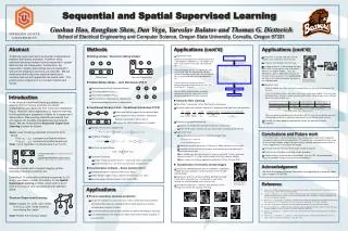
Traditional supervised learning assumes independence between training examples, but many problems involve sequential or spatial data with interdependencies. By exploiting these relationships, prediction accuracy can be improved. This research focuses on developing new methods for machine learning with such data, aiming to enhance classifier performance. Experiment results showcase the effectiveness of sliding window techniques and neural networks in handling sequential and spatial data, with ongoing efforts to further optimize performance. The study delves into techniques like sliding windows, neural networks, and majority voting to classify data accurately in a sequential manner.

Sequential and Spatial Supervised Learning
E N D
Presentation Transcript
Position-Specific Scoring Matrix A R N D C Q E G H I L K M F P S T W Y V Class 1 I -1 -3 -3 -3 -1 -3 -3 -4 -3 4 2 -3 1 0 -3 -2 -1 -3 -1 3 H 2 P -1 -2 -2 -1 -3 -1 -1 -2 -2 -3 -3 -1 -2 -4 7 -1 -1 -4 -3 -2 H 3 A 4 -1 -2 -2 0 -1 -1 0 -2 -1 -1 -1 -1 -2 -1 1 0 -3 -2 0 H 4 Y -2 -2 -2 -3 -2 -1 -2 -3 2 -1 -1 -2 -1 3 -3 -2 -2 2 7 -1 H 5 L -1 -2 -3 -4 -1 -2 -3 -4 -3 2 4 -2 2 0 -3 -2 -1 -2 -1 1 H 6 A 4 -1 -2 -2 0 -1 -1 0 -2 -1 -1 -1 -1 -2 -1 1 0 -3 -2 0 H 7 E -1 0 0 2 -4 2 5 -2 0 -3 -3 1 -2 -3 -1 0 -1 -3 -2 -2 E 8 T 0 -1 0 -1 -1 -1 -1 -2 -2 -1 -1 -1 -1 -2 -1 1 5 -2 -2 0 E 9 L -1 -2 -3 -4 -1 -2 -3 -4 -3 2 4 -2 2 0 -3 -2 -1 -2 -1 1 E 10 Y -2 -2 -2 -3 -2 -1 -2 -3 2 -1 -1 -2 -1 3 -3 -2 -2 2 7 -1 E 11 Y -2 -2 -2 -3 -2 -1 -2 -3 2 -1 -1 -2 -1 3 -3 -2 -2 2 7 -1 E 12 A 4 -1 -2 -2 0 -1 -1 0 -2 -1 -1 -1 -1 -2 -1 1 0 -3 -2 0 C 13 M -1 -1 -2 -3 -1 0 -2 -3 -2 1 2 -1 5 0 -2 -1 -1 -1 -1 1 C 14 K -1 2 0 -1 -3 1 1 -2 -1 -3 -2 5 -1 -3 -1 0 -1 -3 -2 -2 C 15 G 0 -2 0 -1 -3 -2 -2 6 -2 -4 -4 -2 -3 -3 -2 0 -2 -2 -3 -3 C 16 A 4 -1 -2 -2 0 -1 -1 0 -2 -1 -1 -1 -1 -2 -1 1 0 -3 -2 0 C 17 G 0 -2 0 -1 -3 -2 -2 6 -2 -4 -4 -2 -3 -3 -2 0 -2 -2 -3 -3 C 18 T 0 -1 0 -1 -1 -1 -1 -2 -2 -1 -1 -1 -1 -2 -1 1 5 -2 -2 0 C Sequential and Spatial Supervised Learning Guohua Hao, Rongkun Shen, ,Dan Vega, Yaroslav Bulatov and Thomas G. Dietterich School of Electrical Engineering and Computer Science, Oregon State University, Corvallis, Oregon 97331 Applications (cont’d) Abstract Methods Applications (cont’d) Traditional supervised learning assumes independence between the training examples. However, many statistical learning problems involve sequential or spatial data that are not independent. Furthermore, the sequential or spatial relationships can be exploited to improve the prediction accuracy of a classifier. We are developing and testing new practical methods for machine learning with sequential and spatial data. This poster gives a snapshot of our current methods and results. • Sliding window / Recurrent sliding window Experiment result Divide the training data into a sub-training set and a development (validation) set. Try window sizes from 1 to 21 and tree sizes from 10, 20, 30, 50, 70. The best window size was 11, and the best tree size was 20. With this configuration, the best number of iterations to train was 110, which gave 66.3% correct predictions on the development set. Train on the entire training set with this configuration and evaluate on the test set. The result was 67.1% correct. Neural network sliding windows give better performance than this, so we are currently designing experiments to understand why! A classifier is trained, and run on the 8 rotations and reflections of the test set. A majority vote decides the finalclass. A sliding window is used to group the input pixels with varying square size, the same is done for the output window. Thus, the labeling of a pixel is dependent not only on the pixel intensity values in its neighborhood, but also on the labels placed on the pixels in the neighborhood ProteinAA sequence >1avhb-4-AS: IPAYL AETLY YAMKG AGTDD HTLIR VMVSR SEIDL FNIRK EFRKN FATSL YSMIK GDTSG DYKKA LLLLC GEDD yt-1 yt yt+1 Generate raw profile with PSI-BLAST yt-1 yt yt+1 Majority voting xt-1 xt xt+1 xt-1 xt xt+1 Classification result Recurrent Sliding window Sliding window Pixel labels by NaiveBayes IC=1 OC=3 on each of 8 rotations and reflections of the test image • Hidden Markov Model – Joint Distribution P(X,Y) • Experiment result Different window sizes affect not only the computation time, but also the accuracy of the classifier J48 (C4.5) and Naïve Bayes classifiers are the most extensively studied. The results show that Naïve Bayes achieves a higher accuracy with smaller sliding windows, while J48 does better with larger window sizes. Feed into CRF Generalization of Naïve Bayesian Networks Transition probability P(yt|yt-1) Observation probability P(xt|yt) With conditional independence, impractical to represent overlapping features of observations yt-1 yt yt+1 CRF Training and Testing Output Prediction Results Introduction xt-1 xt xt+1 Figure 4 • Semantic Role Labeling In the classical supervised learning problems, we assume that the training examples are drawn independently and identically from some joint distribution P(x,y). However, many applications of machine learning involve predicting a sequence of labels for a sequence of observations. New learning methods are needed that can capture the possible interdependencies between labels. We can formulate this Sequential Supervised Learning problem as follows: Given: a set of training examples of the form (X,Y), where X=(x1,x2,…,xn) a sequence of feature vectors Y=(y1,y2,…,yn) corresponding label sequences Goal: find a classifier h to predict new X as Y=h(X) A2: Accepted-from The official "shared task" of the 2004 Co-NLL conference. For each verb in the sentence, find all of its arguments and label their semantic roles. • Conditional Random Field – Conditional Distribution P(Y|X) A1: thing accepted ( IC = input context; OC = output context ) He would n’t accept anything of value fromthose he was writing about V: verb Extension of logistic regression to sequential data Label sequence Y forms a Markov random field globally conditioned on observation X Removes the HMM independence assumption AM-MOD: modal yt-1 yt yt+1 A0: acceptor AM-NEG: negation When compared to individual pixel classification (59%) it is easy to see that the recurrent sliding window allows for a significant improvement in the accuracy of the classifier. • Currently, the affect bagging and boosting has on the accuracy is under investigation. xt-1 xt xt+1 • Difficulty for the machine learning • Humans use background knowledge to figure out semantic roles • There are 70 various semantic role tags, which makes it computationally intensive • Experiment result • Two forms of feature-inducing in Conditional Random Fields • Regression tree approach • Incremental field growing • 70 different semantic tags to learn. Training set is 9000, whereas test set is 2,000 • Evaluated using F-measure, the harmonic mean between precision and recall of requested argument types. • Both methods got similar performance, F-measure around 65. The best published performance was 71.72, using a simple greedy left to right sequence labeling • Again, simpler non-relational approaches outperform CRF on this task. Why? Potential function of the random field Conclusions and Future work Conditional Probability • In the recent years, substantial progress has already been make to the sequential and spatial supervised learning problems. This poster has attempted to review some of the existing methods and give out our current methods and experiment results in several applications. Future work will include • Develop methods that can handle large number of classes • Discriminative methods using large margin principles • Understand why structural learning methods, such as CRF, do not outperform classical methods in some structural learning problems • Maximize the log likelihood yt-1 yt yt+1 • Vertical relationship: as in normal supervised learning • Horizontal relationship: interdependencies between label variable, can improve accuracy • Parameter Estimation • Iterative scaling and gradient descent – exponential number of parameters • Gradient tree boosting – only necessary interactions among features xt-1 xt xt+1 • Classification of remotely sensed images Acknowledgement Figure 1 • Discriminative methods – Score function f(X,Y) Examples include part of speech tagging, protein secondary structure prediction etc. Extending 1-D observation and label sequences to 2-D arrays, we obtain a similar formulation for the Spatial Supervised Learning problem, where both X and Y have 2-D structure and interdependencies between labels. Assign the crop identification classes (unknown, sugar beets, stubble, bare soil, potatoes, carrots) to pixels in the remotely sensed image We thank the National Science Foundation for supporting this research under grant number IIS-0307592 Averaged perceptron ( Michael Collins et al. 2002 ) Hidden Markov support vector machine (Yasemin Altun et al. 2003 ) Maximum Margin Markov Network ( Ben Taskar 2003 ) Training set and test set are created by dividing the image in half with a horizontal line. The top half is used as the training set, and the bottom half as the testset. Training Set Expansion – rotations and reflections of the training set increase the training set 8 fold. Figure 5: Image with true labels of the classes. Upper part is the training example and the lower part is the testing example Reference Applications • Dietterich, T.G (2002). Machine learning for sequential data: a review. Structural, Syntactic, and Statistical Pattern Recognition (pp. 15-30). New York: Springer Verlag • Lafferty, J., MaCallum, A., & Pereira, F. (2001) Conditional random fields: Probabilistic models for segmenting and labeling sequence data. Proceedings of the 18th International Conference on Machine Learning (pp.282-289). San Francisco, CA: Morgan Kaufmann • Dietterich T. G. , Ashenfelter, A., & Bulatov, Y. (2004) Training Conditional Random Field via Gradient Tree Boosting. Proceedings of the 21st International Conference on Machine Learning (pp 217-224) Banff, Canada • Jones D. T. (1999) Protein Secondary Structure Prediction Based Matrices. J. Mol. Biol. 292:195-202 • Cuff J.A. and Barton G.J. (2000) Application of Multiple Sequence Alignment Profiles to Improve Protein Secondary Structure Prediction. Proteins: Structure, Function and Genetics 40:502-511 • Carreras, X. & Marquez, L. Introduction to the CoNLL-2004 Shared Task: Semantic Role Labeling. Proceedings of CoNLL-2004 • Della Pietra, S., Della Pietra, V. & Lafferty, J. (1997) Inducing features of random fields. IEEE Transactions on Pattern Analysis and Machine Intelligence, 19(4), 380---393. yi+1,j yi+1,j+1 • Protein secondary structure prediction Structural Supervised Learning: Given: A graph G = (V,E), each vertex is an (xv,yv) pair. Some vertexes are missing the y label Goal: Predict the missing y labels Assign the secondary structure classes (a-helix, b-sheet and coil) to protein’s amino acid (AA) sequence, leading to tertiary and/or quaternary structure corresponding to protein functions Use Position-Specific Scoring Matrix profiles to improve the prediction accuracy Use CB513 datasets, with sequences shorter than 30 AA residues excluded, in our experiment yi,j+1 yi,j xi+1,j xi+1,j+1 xi,j xi,,j+1 Figure 2 Figure 6 training set expansion

