Download
1 / 67
670 likes | 688 Views
Discover the intricacies of sorption processes, including linear and Langmuir adsorption models, ion exchange calculations, and thermodynamic speciation-based sorption models. Explore the various assumptions and advantages of each model to better understand sorption dynamics.

E N D
Sorption Reactions Pierre Glynn, USGS, March 2003
Sorption processes • Depend on: • Surface area & amount of sorption “sites” • Relative attraction of aqueous species to sorption sites on mineral/water interfaces • Mineral surfaces can have: • Permanent structural charge • Variable charge
The Linear adsorption model (constant Kd): where q is amount sorbed per weight of solid, c is amount in solution per unit volume of solution; R is the retardation factor, q is porosity, rb is bulk density. Kd is usually expressed in ml/g and measured in batch tests or column experiments. Semi-empirical models • Assumptions: • Infinite supply of surface sites • Adsorption is linear with total element aqueous conc. • Ignores speciation, pH, competing ions, redox states… • Often based on sorbent mass, rather than surface area
Retardation in a fracture: Other linear constant-partitioning definitions (#1) s is amount sorbed per unit surface area; b is fracture aperture; Kf is expressed in L/m2 Non-dimensional partition coefficient: mi is molality of i in the solution or on the surface
Other linear constant-partitioning definitions (#2) Hydrophobic sorption: foc is the fraction of organic carbon (foc should > 0.001); Koc is the partition coeff. of an organic substance between water and 100% organic carbon. Karickoff (1981): Schwartzenbach & Westall (1985): Where a & b are constants (see Appelo & Postma 1993 textbook). KOW is the Octanol-Water partition coeff.
The Langmuir adsorption model: • At the limits: • Kc >> 1 q = b • Kc << 1 q = b Kc where b and Kc are adjustable parameters. Advantages: Provides better fits, still simple, accounts for sorption max. • Assumptions: • Fixed number of sorption sites of equal affinity • Ignores speciation, pH, competing ions, redox states…
The Van Bemmelen-Freundlich adsorption model: where A and b are adjustable parameters with 0 < b < 1 (usually). Advantages: Provides good fits because of 2 adjustable params. Still simple. • Assumptions: • Assumes a log-normal distribution of Langmuir K parameters (I.e. affinities) • Ignores speciation, pH, competing ions, redox states…
Sorption on permanent charge surfaces: • “Ion exchange” • Occurs in clays (smectites), zeolites • Sorption on variable charge surfaces: • “Surface complexation” • Occurs on Fe, Mn, Al, Ti, Si oxides & hydroxides, carbonates, sulfides, clay edges.
Ion Exchange Calcs. (#1) • Involve small cationic species (Ca+2, Na+, NH4+, Sr+2, Al+3) • Exchanger has a fixed CEC, cation exchange capacity • PHREEQC “speciates” the “exchanged species” sorbed on the exchange sites (usually only 1/element); either: • adjusting sorbed concentrations in response to a fixed aqueous composition • or adjusting both sorbed and aqueous compositions
Ion Exchange (#2) • PHREEQC uses 3 keywords to define exchange processes • EXCHANGE_MASTER_SPECIES (component data) • EXCHANGE_SPECIES (species thermo. data) • EXCHANGE • First 2 are found in phreeqc.dat and wateq4f.dat (for component X- and exchange species from Appelo) but can be modified in user-created input files. • Last is user-specified to define amount and composition of an “exchanger” phase.
Ion Exchange (#3) • “SAVE” and “USE” keywords can be applied to “EXCHANGE” phase compositions. • Amount of exchanger (eg. moles of X-) can be calculated from CEC (cation exchange capacity, usually expressed in meq/100g of soil) where: • where sw is the specific dry weight of soil (kg/L of soil), q is the porosity and rB is the bulk density of the soil in kg/L. (If sw = 2.65 & q = 0.3, then X- = CEC/16.2) • CEC estimation technique (Breeuwsma, 1986): • CEC (meq/100g) = 0.7 (%clay) + 3.5 (%organic carbon) • (cf. Glynn & Brown, 1996)
Sorption Exercise (S1) • Change the default thermodynamic database to wateq4f.dat from phreeqc.dat. What are the major differences between both databases? • Use wordpad to look at the thermodynamic data. What are the main ion exchange reactions considered? • How are they written? Does species X- really exist by itself? Is it mobile?
Oklahoma Brine composition: (units are mol/kg water, except mmol/kg water for As; Solution pe must be calculated for equilibrium with atmospheric O2) Sorption Exercise (S2) Enter the above NaCl brine in PHREEQC. Use Cl to charge balance the solution. Equilibrate the brine with 0.1 moles of calcite and 1.6 moles of dolomite. “Save” the resulting solution composition as solution 1. In a new simulation, find the composition of an exchanger X that would be at equilibrium with solution 1 (fixed composition). There is 1 mole of X per kg of water.
Exercise S2 EXCHANGE EQUILIBRIUM_PHASES SOLUTION_SPREAD SAVE
S2 Questions • What happens to the brine as a result of the mineral equilibration? • What is the Na/Ca mole ratio in the brine before and after mineral equilibration? • What is the Na/Ca mole ratio on the exchanger in equilibrium with the calcite and dolomite equilibrated brine? • Bonus: What about the Mg/Ca ratios? What about proton exchange? Are the pH and aqueous concentrations affected by the exchange equilibrium?
S2 Questions (cont) • Re-equilibrate the calcite-and-dolomite equilibrated brine (trhe saved solution 1) with an exchanger that has 0.125 moles CaX2, 0.125 moles MgX2 and 0.5 moles NaX. • How is the aqueous solution affected by the equilibration with the exchanger? • What is the ionic strength of the brine? Is PHREEQC appropriate for this type of calculation? How are the activities of Na+ and Ca+2 species related to their total concentrations • What is the model assumed for the activity coefficients of the sorbed species?
Ion Exchange: thermo. concepts (#1) • Two major issues: • “Activity” definition for “exchanged” species • Convention for heterovalent exchange (eg. Na\Ca or K\Sr) • For homovalent exchange (eg. K\Na), selectivity coefficients usually defined as: • where [i] represents the activity of i.
Ion Exchange: thermo. concepts (#2) • Activities of “exchanged” species calculated either: • as molar fractions • as equivalent fractions • Activity coefficients typically ignored (but not always and Davies and Debye-Huckel conventions can be used in PHREEQC)
Ion Exchange: thermo. concepts (#3) • Heterovalent exchange (eg. Na\Ca): what is the standard state for the exchanged species, Ca0.5X or CaX2 ? In latter case, the law of mass action is: • Both the Gaines & Thomas (default in PHREEQC) and Vanselow conventions use CaX2 as the standard state for divalent Ca on the exchanger. • Gaines & Thomas uses equivalent fractions of exchange species for activities • Vanselow uses molar fractions
Ion Exchange: thermo. concepts (#4) • Gapon convention uses Ca0.5X as the standard state for Ca+2 on the exchanger and uses equivalent fractions for sorbed ion activities. • Gapon convention selectivity coeff. for Na\Ca exchange:
Ion Exchange & Transport (#1) • Selectivity coeffs. are similar to Kd distribution coeffs. (linear adsorption model) when: • one of the elements is present in trace concentrations • the concentrations of major ions remains constant Constant? Constant if q & rB are constant
Ion Exchange & Transport (#2) Unlike most non-linear empirical adsorption isotherms (Langmuir, Freundlich) used in “reactive transport codes”, ion exchange isotherms can be concave upwards, i.e. exhibit greater partitioning at higher concentrations Most isotherms usually result in self-sharpening fronts and smeared-out tails, because of greater sorption at lower concentrations. Ion exchange isotherms can result in smearing fronts.
Ion exchange: final remarks • Selectivity preference on exchangers, generally: • Divalents > monovalents: Ca > Na • Ions w/ greater ionic radius (& consequently lower hydrated radius): Ba > Ca, Cs > Na, heavy metals > Ca • The amount and direction of exchange depends on: • the ratio of ions in solution (and other solution properties) • the characteristics of the exchanger
From Appelo & Postma, 1993, Geochem., groundwater & pollution
Surface Complexation Principles • Fully considers variable charge surfaces. # of sorption of sites is constant but their individual charge, & total surface charge, vary as a function of solution composition • Similar to aqueous complexation/speciation • A mix of anions, cations & neutral species can sorb • Accounts for electrostatic work required to transport species through the “diffuse layer” (similar to an activity coefficient correction) Gouy-Chapman theory
Surface charge depends on the sorption/surface binding of potential determining ions, such as H+. Formation of surface complexes also affects surface charge.
Examples of Surface Complexation Reactions outer-sphere complex inner-sphere complex bidentate inner-sphere complex
Gouy-Chapman Double-Layer Theory The distribution of charge near a surface seeks to minimize energy (charge separation) and maximize entropy. A charged surface attracts a diffuse cloud of ions, preferentially enriched in counterions. The cation/anion imbalance in the cloud gradually decreasses away from the surface.
The Double-Layer model assumes: • a surface layer of charge density s and uniform potential Y throughout the layer • a “diffuse” layer of total charge density sd with exponentially decreasing potential away from the surface layer Electroneutrality requires that: The charge density of the surface layer is determined by the sum of protonated and deprotonated sites and sorbed charged complexes: Where F is the Faraday const. (96490 C/mol), A is the spec. surf. area (m2/g), S is the solid concentration (g/L), ms and ns are the molar concentrations and charges of surface species.