Download
1 / 39
390 likes | 567 Views
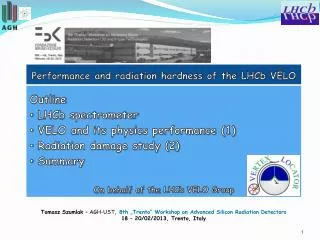
Performance and radiation hardness of the LHCb VELO. Outline LHCb spectrometer VELO and its physics performance (1) Radiation damage study (2) Summary On behalf of the LHCb VELO Group.

E N D
Performance and radiation hardness of the LHCb VELO • Outline • LHCb spectrometer • VELO and its physics performance (1) • Radiation damage study (2) • Summary • On behalf of the LHCb VELO Group Tomasz Szumlak – AGH-UST, 8th „Trento” Workshop on Advanced Silicon Radiation Detectors 18 – 20/02/2013, Trento, Italy
TT+IT (Silicon Tracker) Muon system 300/250 mrad OT Dipole magnet Calorimeters Vertex Locator 15mrad RICH detectors LHCb is a dedicated flavour experiment with the main focus on CP-violation and New Physics in b- and c-mesons Must provide: excellent position, vertex and momentum resolution & PID A forward spectrometer is sufficient for the LHCb physics programme since produced b-bbar pairs are strongly correlated and forward peaked Interaction Point OT – Outer Tracker IT – Inner Tracker TT – Trigger Tracker
Operation conditions of the LHCb in 2012 • Beam energy = 4.0 [TeV] (15 % increase of the b-bbar x-section w.r.t. 2011) • Keep the luminosity at Linst = 4.0 x 1032 [cm-2s-1 ] • Average number of visible interactions per x-ing slightly higher µ = 1.6 • HLT (High Level Trigger) input ~ 1.0 MHz, output ~ 5 kHz (upgraded HLT farm and revisited code) • Over 2 fb-1 of p-p collision data recorded between 2010 and 2012
Operation conditions of the LHCb in 2012 • Beam energy = 4.0 [TeV] (15 % increase of the b-bbar x-section w.r.t. 2011) • Keep the luminosity at Linst = 4.0 x 1032 [cm-2s-1 ] • Average number of visible interactions per x-ing slightly higher µ = 1.6 • HLT (High Level Trigger) input ~ 1.0 MHz, output ~ 5 kHz (upgraded HLT farm and revisited code) • Over 2 fb-1 of p-p collision data recorded between 2010 and 2012 6
The RUN I officially finished on 14/02/2013 LHCb spectrometer, in general, and the VELOin particular performed SUPERBLY Both – the detector and its infrastructure werepushed to the limits surpassing any initial expectations Will be back in 2015…
The VELO performance • Basic requirements and design • Signal and noise • Time and spatial alignment • Single hit resolution (spatial resolution) • Vertex and IP resolutions • Velo tomography with hadronic vertices • Summary
Design and requirements • Base-line requirements • extreme hadronic radiation environment due to VELO closeness to the beam • first active strips at ~ 8 mm • particle fluence of up to 5x10¹³ 1 MeVneq/cm2/1 fb-1 • small material budget (sensor thickness 300 µm) • high intrinsinc spatial resolution (analogue readout & fine strip pitch: ~ 40 – 100 µm) • What do we want from the VELO • primary and secondary (displaced) vertex reconstruction • b- and c-hadrons lifetime measurement - O(10-12) s • impact parameter (IP) ~ mm • flight distance ~ cm • vital part of the HLT (software High Level Trigger)
y x z pile-up modules injection p LHC vacuum stable beams Modules (21+2) RF box p - 2 retractable detector halves:~8 mm from beam when closed, retracted by 30mm during injection - 21 tracking stations per detector half - Secondary vacuum tank - 300μm foil separates detector from beam vacuum - Evaporative, bi-phase C02 cooling system - Nominal operational temp. -8o C (silicon) - Pile-up modules provide on-line input to the trigger
r=42 mm r=8 mm 2048 strips • Surrounds the LHCb luminous region • Unique R-Φ geometry with floating 40–100 μm strip pitch • Each module (R+Φ) mounted on carbon fiber support paddle • Oxygenated n+-on-on sensors (one pair of n+-on-p) • Optimized for • tracking of particles originating from beam-beam interactions • fast 3D tracking done on-line ~ 1 m RF foil 3cm separation interaction point pile-up veto (R-sensors) R
Signal and noise - Typical noise measured in the VELO close to 2 ADC counts - Signal to noise after 2 years of operation S/N over 19 - Stable over time (2010 – 2012)
Time and spatialalignment • - The purpose of the time alignment • - Set the ADC sampling time (digitisation of the analogue signal) • - Optimise S/N, minimise bunch cross-talk • - Spatial alignment • - Precise assembly • - Mechanical and optical survey • - Software alignment with tracks • - Closely monitored, stable over time
Single hit resolution • - Intrinsic spatial resolution • - Combination of fine strip pitch and analogue read-out • - Multi-strip clusters improves the resolution • - The resolution described in an abstract 2D parameter space • - Projected angle (strip geometry), θp • - Strip pitch, P • - Best spatial resolution at the LHC ~ 4µm (for optimal P and θp)
Vertex resolution • - Vertex resolution, PV, parametrised as function of the number of track – N • - Consistent with the design performance • - Some degradation observed as a function of pile-up (more than one PV per beam crossing) • - Performance for N=25 • - X/Y ~ 13 µm • - Z ~ 69 µm
Impact Parameter resolution • - Impact parameter (IP) is defined as a perpendicular distance between a particle's trajectory (track) and a fixed point in space (usually the PV) • - The IP resolution is driven by: • - Single hit resolution • - Distance between the PV and the first measurement • - Multiple scattering • - IP = 13.2 + 24.7/pT µm
VELO imaging - tomography • - VELO „tomography” • - Use vertices from hadronic interaction with the detector material • - Build the material map based on the vertices distribution • - Precise material description is vital for IP measurement
The VELO performance - Summary • Great overall performace of the VELO in 2010 – 2012 • S/N ~ 18 • Best spatial resolution ~ 4 µm • Impact parameter resolution IP = 13.2 + 24.7/pTµm • PV resolutions: Ip(x,y) = 13 µm, Ip(z) = 69 µm
Radiation hardness of the VELO • Study of leakage current vs. temperature (IT scan) • Effective depletion voltage (EDV) • Cluster finding efficiency measurement • Second metal layer effect
VELO sensors revisited n+-on-n type (82) - Depletion region grows from the backplane toward the junction - Type inversion (space charge sign) after ~ 1012 neq/cm2 - p-spray for inter-strip isolation n+-on-p type (2) - Depletion region grows from the strip implant towards backplane - No type inversion - p-spray for inter-strip isolation - n-strip readout via capacitively coupled first metal layer - routing lines (second metal layer) connect strips with the readout front-end
IT scans • - Bulk and surface currents • - Bulk or surface dominated sensor are present • - Influence of the surface component after irradiation is negligible • - Fitting the data points with the exponential model allows to measure the effective band gap Eg
Currents evolution • - Bulk current increase with fluence, i.e., delivered luminosity • - Trend plot (current as a function on time) • - The mean value of bulk current follows the MC predictions • - The leakage current vs. sensor coordinate along the beam line • - Scaled to the common temp. 21o C • - Good agreement with the simulation
Effective depletion voltage (EDV) - Type inversion expected for n+-on-n - Initial drop of the VFD for n+-on-p sensors followed by increase - C-V scans used to perform the initial measurements for the VELO during the detector assembly - Once the system is operational this cannot be repeated - Alternative method is needed
Charge collection efficiency (CCE) • - „Unbiased” information using tracks • - exclude tested sensors from the track fit • - perform the voltage scan (0 – 150 V) for them • - measure the charge deposited within a window around the track intercept • - Plot the MPV value of the fitted Landau vs. bias voltage
Charge collection efficiency (CCE) - Initial decrease of the VFD with delivered luminosity confirmed! - Inner part of the VELO sensors (low radius) is type inverted - The minimal value of the VFD ~ 20 V - Inversion at ~ 10 – 15 x 1012neq - Is the Hamburg model valid? Let’s compare!
Charge collectionefficiency (CCE) - Comparison with the Hamburg model for different voltages - Reasonably good agreement with the model - A significant departure from what the model predicts only around inversion point - But this is hard to measure – need a sufficient electric field to collect the charge
Cluster finding efficiency (CFE) - It was found that R-type sensors show drop in CFE that depends on their position w.r.t the interaction point - No significant effect related to -type ones - This is quite unexpected - A detailed investigation has been performed…
Clusterfindingefficiency (CFE) - A detailed analysis for a selected downstream R-type sensor (#34) with large amount of data performed - Effect depends on delivered luminosity - Increasing the bias voltage did not help – on the contrary it made things worse - This was also unexpected…
Second metal layer effect Routing lines map for R-type sensors • - An interesting observation has been made during the analysis • - CFE drops as a function of fluence • - The outer radial region suffers the most • - Looks like high CFE is preserved if no routing lines are present CFE after ~ 40 pb-1 of data CFE after ~ 1.2 fb-1 of data
Second metal layer - revisited Small R LargeR • - 1st metal layer coupled to the strips, 2nd metal layer transport signals to the FE • - Different strip geometries – routing lines are • - perpendicular to strips in R-type sensors • - parallel to strips in -type sensors • - Charge can capacitively couple to routing lines in R-type sensors • - Fake cluster generation (see next slide) and CFE drop
Second metal layer effect - CFE is worst when a hit is far fromstrips and close to routing lines - This is clearly visible when plotting the ‘raw signal’ - Fortunately this is no correlation between sensors, thus, no visible effect observed for ‘clusters on track’
Radiation hardness of the VELO Summary • A number of analyses ongoing to monitor and study radiation damage effects for the LHCb VELO • Changes in EDV follow the expectations • Drop in CFE due to second metal layer effect observed for R-type sensors • No visible degradation in tracking performance though • A paper regarding these studies sent out for publication
Physics motivation for the LHCb experiment • study flavour changing and CP violating processes in b- and c-quark sector • search for New Physics signatures therein • Indirect approach (or probing intensity frontier) complementary to Atlas and CMS • study higher order box or penguin processes (i.e., that proceed via loop diagrams) • highly sensitive to new states that can appear at high mass scale • strongly suppressed (and well predicted) in the SM • Perform precise measurements and look for deviations w.r.t. the theory
TT+IT (Silicon Tracker) Muon system 300/250 mrad OT Dipole magnet Calorimeters Vertex Locator 15mrad RICH detectors The LHCb is a forward spectrometer, angular acceptance 15 – 300 (250)mrad or in other ‘pseudo-rapidity language’ η = 1.9 - 4.9 Mustprovide: excellentposition, vertex and momentum resolution & PID A forward spectrometer is sufficient for the LHCb physics programme since produced b-bbarpairs are strongly correlated and forward peaked General Purpose experiment for the forward region Interaction Point OT – OuterTracker IT – InnerTracker TT – TriggerTracker
Operation conditions of the LHCb in 2012 • Beam energy = 4.0 [TeV] (15 % increase of the b-barb x-section) • Keep the luminosity at Linst = 4.0 x 1032 [cm-2s-1 ] for this year • Average number of visible interactions per x-ing slightly higher µ = 1.6 • Keep high data taking efficiency and quality • HLT (High Level Trigger) input ~ 1.0 MHz, output ~ 5 kHz (upgraded HLT farm and revisited code) • Expecting ~ 1.5 fb-1 of recorded data by the end of the year
Time alignment • - Proper setting of the timing and gain are critical for: • - Cross-talk effects between channels in the same link • - Uniformity of pedestals and noise • - Calibration of the signal levels measured • - Vital for setting the timing of the pulse sampling with respect to the LHC beam 37
Spatial alignment • - Very tight requirements on the VELO alignment • - Intrinsic hit resolution • - Impact parameter • - Decay time resolution • - VELO halves are inserted and centred on the beams for each fill • - Closing procedure is fully automated • - On-line update of the alignment parameters for the HLT • - Stability evaluated by fitting the PV for each half separately
Spatial alignment • - Software based alignment • - Track residuals based • - Relative sensor alignment • - Relative alignment of the modules • - VELO halves alignment • - Sensor misalignment is of the order of 4 µm • - The overall alignment depends on • - Precise assembly • - Mechanical and optical survey • - Software alignment with tracks