Download
1 / 37
370 likes | 585 Views
Using Ion Source Beam Measurements in GPT. Simon Jolly Imperial College FETS Meeting, 12/10/05. LEBT Optimisation. To effectively optimise LEBT, must have accurate model of beam at start of LEBT ie. at source extraction.

E N D
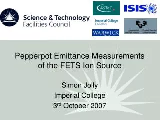
Using Ion Source Beam Measurements in GPT Simon Jolly Imperial College FETS Meeting, 12/10/05
LEBT Optimisation • To effectively optimise LEBT, must have accurate model of beam at start of LEBT ie. at source extraction. • In an ideal world, we could take measurements of the ion source beam profile and emittance at extraction and feed this directly into GPT. • Not so simple: only emittance profiles from Ion Source (Dan Faircloth); GPT needs single particle x-x’ and y-y’ data. • 2 options: data interpolation or built-in GPT functions.
Ion Source Measurements • Measurements made 600mm downstream from Ion Source (DF): • Hrms = 0.92, Vrms = 1.01 mm mrad. • xrms = 26.0 mm, x’rms = 32.0 mrad. • yrms = 24.6 mm, y’rms = 35.0 mrad. • Previously, data approximated in GPT using built-in particle distributions: uniform in x/x’, quadratic in y/y’. • Results unsatisfactory (so far), particularly with reverse simulations: 4D correlation not possible.
Ion Source Emittance Horizontal and Vertical emittance measurements
GPT Ion Source Emittance X & Y emittance profiles produced by GPT Y X
Ion Source X/X’ Profiles Horizontal emittance profiles X X’
Ion Source Y/Y’ Profiles Vertical emittance profiles Y Y’
Raw Emittance Data Need to produce input file for GPT from DF measured data. Start with raw data file (histogram data)…
Matlab Interpolation Convert histogram data into individual particle data: use random distribution of points for each phase space cell (increases emittance)…
Particle Set Reduction Reduce number of particles to 10,000 total to produce suitable number for GPT input…
Recalculate Emittance Reproduce histogram for beam distribution compare to real data. Data could now be input to GPT.
Real Emittance Real data
Not so fast… However, while x-x’ and y-y’ now produce correct particle distributions, x-y does not! Need to find a way to input correlated x-y distribution.
X-Y Histogram: Real Data No measured data on real x-y distribution: have to construct it. Multiply x & y profiles together to produce reconstructed x-y profile.
Ion Source X/Y Profiles Beam position profiles (from data) X Y
Make Particle X-Y Correlation Divide x-y profile into grid according to phase space cells from emittance plots. Distribute particles into phase space cells.
Correlated X-Y Distribution Distributing previously created particles according to x-y profiles gives a beam profile one can input into GPT (10,000 particles).
Correlated X-Y Profile Histogram of 10,000 correlated particles.
Correlated X-Y Profile (100k) Histogram of 100,000 correlated particles.
Real X-Y Profile X-Y profile from measured data.
Random X-Y Correlation Just as a sanity check: randomly distribute particles and produce histogram of 10,000 uncorrelated particles.
GPT Input • We now have a 4-D correlated particle set to input to GPT. Distributions also centred - is this necessary? • Treat set as mono-energetic 2D slice at 600mm, input to GPT and run backwards using SCtree2D space charge model. • Try to match x-y profile at 0mm to real exit aperture of cold box, using different space charge compensation.
Results: Input Data (X-Y) X-Y plot for initial beam data.
Results: X-Y, 10% SC X-Y plot for beam at 0mm, 10% space charge.
Results: X-Y, 20% SC X-Y plot for beam at 0mm, 20% space charge.
Results: X-Y, 30% SC X-Y plot for beam at 0mm, 30% space charge.
Results: X-Y, 40% SC X-Y plot for beam at 0mm, 40% space charge.
Results: X-Y, 50% SC X-Y plot for beam at 0mm, 50% space charge.
Results: Input Data (Emit) Emittance plots for initial beam data
Results: Emittance, 10% SC Emittance plots for beam at 0mm, 10% space charge X Y
Results: Emittance, 20% SC Emittance plots for beam at 0mm, 20% space charge X Y
Results: Emittance, 30% SC Emittance plots for beam at 0mm, 30% space charge X Y
Results: Emittance, 40% SC Emittance plots for beam at 0mm, 40% space charge X Y
Results: Emittance, 50% SC Emittance plots for beam at 0mm, 50% space charge X Y
Mafia Data Simulation Input position & velocity data of 10,000 particles to GPT, generated from Mafia simulation (DF). X Y
Results • We now have a method of producing a beam for GPT simulations from real data. • Simulations show differences between different levels of space charge compensation for the ion source beam. • Factor of 2 in x/y depending upon space charge compensation.
Still to do… • Fine tune space charge compensation to match real exit aperture of cold box. • Use “idealised” custom distribution as input for GPT and try to reproduce measured results - get rid of measurement artifacts. • Input “best beam” to LEBT optimisation simulation.