Presentation AUV Data Analysis
Presentation AUV Data Analysis. MAR 670 Anne-Marie E.G. Brunner. Introduction Data Methods for Project III The Plan Methods Results Summary. 1. Introduction. Turbulence Remus. Upper CTD. Lower CTD. Shear probe FP07 thermistor. ADV. Upward and Down ward ADCPs.

Presentation AUV Data Analysis
E N D
Presentation Transcript
PresentationAUV Data Analysis MAR 670 Anne-Marie E.G. Brunner
Introduction • Data • Methods for Project III • The Plan • Methods • Results • Summary
Turbulence Remus Upper CTD Lower CTD Shear probe FP07 thermistor ADV Upward and Down ward ADCPs
AUV Probe – the Data Z b3 Note: this is a left-handed Coordinate system! X b1 Y b2 We only measure water-acceleration to the right and left, and up and down.
*Data have been collected in a passage in Narragansett Bay.*76s of data at a sampling frequency of 1024Hz leads to 77825 data points.*We have measurements of accelerations relative to the bottom – a fixed coordinate system – bx, by, bz using an accelerometer.*All three vehicle body accelerations are contaminated by noise mi. The noise is considered to be independent of the other instruments noise.*The water acceleration is measured in y and z with a shear probe relative to the AUV: uy, uz; these data are also contaminated by noise ni, and again the noise is assumed to be independent of each other and the noise caused by the vehicle acceleration noise.*We further assume, that uy and uz are not correlated as will be shown later.*A schematic will follow.
All noise is independent of each other and independent of the measured quantities.If the vehicle body accelerations are zero, and all noise is zero, the shear probe would measure the non-contaminated water acceleration.
The three Projects • From acceleration find velocities • The single input case – assume u1dot is only contaminated by b2 and u2dot by b3: Single input – single output. • Assume uy is contaminated by bx, by and bz: multiple input single output.
Review of the Mathematics Fourier-transform (handeling of convolution) the equation to estimate the transfer-function between input and output signals. Use this transfer-function to estimate the decontaminated Outputspectra.
The Equation for the estimated Spectra Transfer-function For Matlab those matrices have 3 dimension with up to 3x3xNo.of Harmonics
“Plan for Project” • Low-pass-filtering of the original data with a cutoff frequency of 32Hz. The Nyquist-frequency is 512Hz. Decimating at 128Hz to reduce the volume of the data (time series contains originally 77825 points) and speed up the calculations. • Applying the filter to a random set of data. • Computing auto-spectra and cross-spectra, according to the theory discussed earlier on, especially the decontaminated spectra. • Plot also as variance preserving. • Uncertainty limits • Testing of the Assumptions if possible • Interpretation of results: comparison with the random result, if chance, comparison to SISO results, physical/oceanographic context of results if possible.
5. Methods A matlab code was developed to obtain the following graphs and results. The mean was taken out. The data have been low-pass filtered with an order 4 butterworth-fitler, and fcut=32Hz. csd, psd, cohere (implemented Matlab functions) were used for the caculation
DOF The original TimeSeries had 77825 points at a sampling frequency of 1024Hz, the decimated reduced to 9728 points and a sampling frequency of 128Hz (fnyquist=64Hz). The section length was 1024 and therefore there were 9 sections; DOF=2*9=18. There are 513 harmonics.
Autospectra Inputs, uncorrected Output Peaks at 18Hz and 38Hz
UzUz and UyUy spectra green and blue are corrected
UzUz and UyUy spectra variance preserved green and blue are corrected Most Variance occurs in the band between 5Hz and 20Hz.
Fcut Fcut
Summary • Uy and Uz can be assumed as uncorrelated as was assumed for this analysis • The MISO analysis shows that the distinct ~20Hz (0.05s) peak is not seen in the decontaminated output spectra and it is suspected to be caused by the vehicle movement. • The 5Hz to 20Hz frequency band (0.05s-0.2s) is the most energetic for the decontaminated acceleration spectra. This means the water-acceleration is most energetic for this band. This frequency range is typical for capillary waves (wind), or maybe even ultra-gravity waves (gravity) or other sources.
Problems and Future thoughts • Although the time-series were filtered at Fcut=32Hz significant peak and coherence is found at 38Hz for the input-autospectra; similar things were seen in the coherences between output and input spectra. • A comparison with the SISO dataset was not possible at this point.
A short Overview over the Mathematics and Theory The Overall Goal: Determining the decontaminated or corrected Water Acceleration Spectra.
The difference between the estimated and the true spectrum will give the error, dividing this result by the estimated spectrum leads to the delta. The total error is : <delta^2>= random error-biased error= <(delta-<delta>)^2+<delta>^2