Download
1 / 68
680 likes | 881 Views
Global Constraints: Generalised Arc Consistency. It is often important to define n-ary “global” constraints, for at least two reasons Ease the modelling of a problem

E N D
Global Constraints: Generalised Arc Consistency • It is often important to define n-ary “global” constraints, for at least two reasons • Ease the modelling of a problem • Exploitation of specialised algorithms that take the semantics of the constraint for efficient propagation, achieving generalised arc consistency. • The generalised arc consistency (GAC) criterion sees that no value remains in the domain of a variable with no support in values of each of the other variables participating in the “global” constraint. Example:all_diff ([A1, A2, ..., An] Constrain a set of n variables to be all different among themselves
all_diff([]). • all_diff([H|T]):- • one_diff(H,T), • all_diff(T). • one_diff(_,[]). • one_diff(X,[H|T]):- • X #\= H, one_diff(X,T). Global Constraints: all_diff • The constraint definition based on binary difference constraints () does not pose any problems as much as modelling is concerned. For example, it may be being defined recursively in CLP. • However, constraint propagation based on binary constraints alone does not provide in general much propagation. • As seen before, arc consistency is not any better than node consistency, and higher levels of consistency are in general too costly and do not take into account the semantics of the all_different constraint.
Global Constraints: all_diff Example: X1: 1,2,3 X6: 1,2,3,4,5,6,7,8,9 X2: 1,2,3,4,5,6 X7: 1,2,3,4,5,6,7,8,9 X3: 1,2,3,4,5,6,7,8,9 X8: 1,2,3 X4: 1,2,3,4,5,6 X9: 1,2,3,4,5,6 X5: 1,2,3 • It is clear that constraint propagation based on maintenance of node-, arc- or even path-consistency would not eliminate any redundant label. • Yet, it is very easy to infer such elimination with a global view of the constraint!
Global Constraints: all_diff • Variables X1, X5 and X8 may only take values 1, 2 and 3. Since there are 3 values for 3 variables, these must be assigned these values which must then be removed from the domain of the other variables. • Now, variables X2, X4 and X9 may only take values 4, 5 e 6, that must be removed from the other variables domains. X1: 1,2,3 X2:1,2,3,4,5,6 X3:1,2,3,4,5,6,7,8,9 X4:1,2,3,4,5,6 X5: 1,2,3 X6:1,2,3,4,5,6,7,8,9 X7:1,2,3,4,5,6,7,8,9 X8: 1,2,3 X9:1,2,3,4,5,6 X1: 1,2,3 X2:1,2,3,4,5,6 X3:1,2,3,4,5,6,7,8,9 X4:1,2,3,4,5,6 X5: 1,2,3 X6:1,2,3,4,5,6,7,8,9 X7:1,2,3,4,5,6,7,8,9 X8: 1,2,3 X9:1,2,3,4,5,6
Global Constraints: all_diff • In this case, these prunings could be obtained, by maintaining (strong) 4-consistency. • For example, analysing variables X1, X2, X5 and X8, it would be “easy” to verify that from the d4 potential assignments of values to them, no assignment would include X2=1, X2=2, nor X2=3, thus leading to the prunning of X2 domain. • However, such maintenance is usually very expensive, computationally. For each combination of 4 variables, d4 tuples whould be checked, with complexity O(d4). • In fact, in some cases, n-strong consistency would be required, so its naïf maintenance would be exponential on the number of variables, exactly what one would like to avoid in search!
Global Constraints: all_diff • However, taking the semantics of this constraint into account, an algorithm based on quite a different approach allows the prunings to be made at a much lesser cost, achieving generalised arc consistency. • Such algorithm (see [Regi94]), is grounded on graph theory, and uses the notion of graph matching. • To begin with, a bipartite graph is associated to an all_diff constraints. The nodes of the graphs are the variables and all the values in their domains, and the arcs associate each variable with the values in its domain. • In polinomial time, it is possible to eliminate, from the graph, all arcs that do not correspond to possible assignments of the variables.
Global Constraints: all_diff Key Ideas: • For each variable-value pair, there is an arc in the bipartite graph. • A matching, corresponds to a subset of arcs that link some variable nodes to value nodes, different variables being connected to different values. • A maximal matching is a matching that includes all the variable nodes. • For any solution of the all_diff constraint there is one and only one maximal matching.
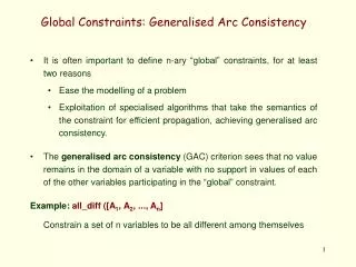
Maximal Matching 1 A B D 2 A = 1 B = 2 C = 3 D = 4 E = 5 C E 3 4 5 6 Global Constraints: all_diff Example:A,B:: 1..2, C:: 1..3, D:: 2..5, E:: 3..6, all_diff([A,B,C,D,E]).
Global Constraints: all_diff • The propagation (domain filtering) is done according to the following principles: • If an arc does not belong to any maximal matching, then it does not belong to any all_diff solution. • Once determined some maximal matching, it is possible to determine whether an arc belongs or not to any maximal matching. • This is because, given a maximal matching, an arc belongs to any maximal matching iff it belongs: • To an alternating cycle; or • To an even alternating path, starting at a free node.
1 A B D 2 3 C E 4 5 6 Global Constraints: all_diff • 6 is a free node; • 6-E-5-D-4 is an even alternating path, alternating arcs from the MM (E-5, D-4) with arcs not in the MM (D-5, E-6); • A-1-B-2-A is an alternating cycle; • E-3 does not belong to any alternating cycle • E-3 does not belong to any even alternating path starting in a free node (6) • E-3may befiltered out! Example: For the maximal matching (MM) shown
Global Constraints: all_diff • Compaction • Before this analysis, the graph may be “compacted”, aggregating, into a single node, “equivalent nodes”, i.e. those belonging to alternating cycles. • Intuitively, for any solution involving these variables and values, a different solution may be obtained by permutation of the corresponding assignments. • Hence, the filtering analysis may be made based on any of these solutions, hence the set of nodes can be grouped in a single one.
A/B 1/2 1 D A B 3 2 C E C D/E 4/5 3 6 4 5 6 Global Constraints: all_diff • A-1-B-2-A is an alternating cycle; • By permutation of variables A and B, the solution <A,B,C,D,E> = <1,2,3,4,5> becomes <A,B,C,D,E> = <2,1,3,4,5> • Hence, nodes A e B, as well as nodes 1 and 2 may be grouped together (as may the nodes D/E and 4/5). With these grouping the graph becomes much more compact
A/B 1/2 3 C C D/E 4/5 6 A/B 1/2 3 D/E 4/5 6 Global Constraints: all_diff • Arc D/E - 3 may be filtered out (notice that despite belonging to cycle D/E - 3 - C - 1/2 - D/E, this cycle is not alternating. • Arcs D/E - 1/2andC - 1/2may also be filtered. Analysis of the compacted graph shows that The compact graph may thus be further simplified to
1 2 A D B 3 4 C C E 5 6 A/B 1/2 3 D/E 4/5 6 Global Constraints: all_diff By expanding back the simplified compact graph, one gets the graph on the rightthat Which immediately sets C=3 and, more generaly, filters the initial domains to A,B :: 1..2, C:: 1,2,3, D:: 2,3,4,5, E:: 3,4,5,6
1 2 D A B B D A 3 1 4 C C E E 2 5 ? 3 6 4 5 6 Global Constraints: all_diff • Upon elimination of some labels (arcs), possibly due to other constraints, the all_diff constraint propagates such prunings, incrementally. There are 3 situations to consider: • Elimination of a vital arc (the only arc connecting a variable node with a value node): The constraintcannot be satisfied.
A B D D B A 1 2 C C E E 1 3 2 4 3 5 4 6 5 6 Global Constraints: all_diff • Elimination of a non-vital arc which is a member to the maximal matching • Determine a new maximal matching and restart from there. Arc A-4does not belong to the even alternating path started in node 6. D-5 also leaves this path, but it still belongs to an alternating cycle.
D A B D B A 1 1 2 2 C C E E 3 3 4 4 5 5 6 6 Global Constraints: all_diff • Elimination of a non-vital arc which is not a member to the maximal matching • Eliminate the arcs that do not belong any more to an alternating cycle or path. A new maximal matching includes arcs D-5 and E-6. In this matching, arcs E-4 and E-5do not belong to even alternating paths or alternating cycles.
Global Constraints: all_diff Time Complexity: Assuming n variables, each of which with d values, and where D is the cardinality of the union of all domains, • It is possible to obtain a maximal matching with an algorithm of time complexity O(dnn). • Arcs that do not belong to any maximal matching may be removed with time complexity O( dn+n+D). • Taking into account these results, we obtain complexity of O(dn+n+D+dnn). Since D < dn, the total time complexity of the algorithm is dominated by the last term, thus becoming O(dnn). which is much better than the poor result with a naïf analysis.
Global Constraints: all_diff Availability: • The all_diff constraint first appeared in the CHIP system (algorithm?). • The described implementation is incorporated into the ILOG system, and avalable as primitive IlcAllDiff. • This algorithm is also implemented in SICStus, through buit-in constraint all_distinct/1. • Other versions of the constraint, namely all _different/2, are also available, possibly using a faster algorithm but with less pruning, where the 2nd argument controls the available pruning options.
Global Constraints: all_diff Availability: • The all_diff constraint first appeared in the CHIP system (algorithm?). • The described implementation is incorporated into the ILOG system, and avalable as primitive IlcAllDiff. • This algorithm is also implemented in SICStus, through buit-in constraint all_distinct/1. • Other versions of the constraint, namely all _different/2, are also available, possibly using a faster algorithm but with less pruning, where the 2nd argument controls the available pruning options.
Global Constraints: all_diff • Example: Sudoku • Cuts in green are all that are found by maïve all_diff. • Global all_diff finds all values without backtracking. • The first cuts are illustrated in the figure. • (where the indices show a possible order in which the cuts are made) • sudoku_cp.pl • Files vh1 e vh2
Global Constraints: Assignment • The all_diff constraint is typically applicable to problems where it is intended that different tasks are executed by different agents (or use different resources). • However, tasks and resources are treated differently. Some are variables and the others the domains of these variables. For example, denoting 4 tasks/resources by variablesTi / Rj, one would have to chose either one of the specifications below T1 in 1..3, T2 in 2..4, T3 in 1..4, T4 in 1..3. or R1 in {1,3,4}, R2 in 1..4, R3 in 1..4, R4 in {2,3} • Hence, other constraints could be specified either on tasks or on resources, but not easily involving both types of objects
Global Constraints: Assignment • Such “unfairness” may be overcome by treating both tasks and resources in a similar way, namely modelling both with distinct variables. • These variables still have to adhere to the constraint that different tasks are performed in different resources. • Also, if a task j is assigned to resource i, then resource i is assigned to task j. Denoting tasks by Tj and resources by Ri, the following condition must stand for any i, j 1..n Ri = j Tj = i • This is the goal of global constraint assignment/2, available in SICStus, that uses the same propagation technique of all_diff.
A1 A2 A3 A4 A5 B1 B2 B3 B4 B5 Global Constraints: Assignment Example: A1:1..2, A2::1..2, A3::1..3, A4::2..5, A5:: 3..5, B1:1..3, B2::1..4, B3::3..5, B4::4..5, B5:: 4..5, assignment([A1,A2,A3,A4,A5], [B1,B2,B3,B4,B5]). A = 1 B = 2 C = 3 D = 4 E = 5 maximal matching
A1 A2 A3 A4 A5 B4 B5 B2 B3 B1 A1 B1 B2 A2 A3 B3 A4 B4 A5 B5 Global Constraints: Assignment Since the assignment constraint imposes a maximal matching in the bipartite graph of tasks Ai and Resources Bj and resources, the same filtering techniques of the all_diff constraint can be used. Hence the initial domains are are filtered to A1:1..2, A2::1..2, A3:: 3 , A4::4..5, A5:: 4..5. B1:1..2, B2::1..2, B3:: 3 , B4::4..5, B5:: 4..5.
Global Constraints: Circuit • The previous global constraints may be regarded as imposing a certain “permutation” on the variables. • In many problems, such permutation is not a sufficient constraint. It is necessary to impose a certain “ordering” of the variables. • A typical situation occurs when there is a sequencing of tasks, with precedences between tasks, possibly with non-adjacency constraints between some of them. • In these situations, in addition to the permutation of the variables, one must ensure that the ordering of the tasks makes a single cycle, i.e. there must be no sub-cycles.
C A C A D B D B 2 2 3 6 8 4 2 5 7 2 9 Global Constraints: Circuit • These problems may be described by means of directed graphs, whose nodes represent tasks and the directed arcs represent precedences. • The arcs may even be labelled by “features” of the precedences, namely transition times. • This is a situation typical of several problems of the travelling salesman type.
A C A C B D B D Global Constraints: Circuit • Filtering: For these type of problems, the arcs that do not belong to any hamiltoniancircuit should be eliminated. • In the graph, it is easy to check that the only possible circuits are A->B->D->C->A and A->C->D->B->A. Certain arcs (e.g. B->C, B->B, ...),may not belong to any hamiltoniancircuit and can be safely pruned.
A/1 C/3 B/2 D/4 A=2 A=3 Global Constraints: Circuit • The pruning of the arcs that do not belong to any circuit is the goal of the global constraint circuit/1, available in SICStus. • This constraint is applicable to a list of domain variables, where the domain of each corresponds to the arcs connecting that variable to other variables, denoted by the order in which they appear in the list. For example: A in 2..3,B in 1..4, C in 1..4, D in 2..3, circuit([A,B,C,D]).
A C A C B D B D Global Constraints: Circuit A, D in 2..3,B in 1,2,3,4, C in 1,2,3,4, circuit([A,B,C,D]). • Global constraint circuit/1incrementally achieves the pruning of the arcs not in any hamiltonian circuit. For example, posing The following prunning is achieved A in 2..3,B in 1,2,3,4, C in 1,2,3,4,D in 2..3, since the possible solutions are [A,B,C,D] = [2,4,3,1] and [A,B,C,D] = [3,1,4,2]
A/1 C/3 B/2 D/4 2 2 3 6 8 4 2 5 7 2 9 Global Constraints: Element Often a variable not only has its values constrained by the values of other variables, but it is actually defined conditionally in function of these values. For example, the value X from the arc that leaves node A, depends on the arc chosen: if A = 2 then X = 3, if A = 3 then X = 4; otherwise X = undefined The disjunction implicit in this definition raises, as well known, problems of efficiency to constraint propagation.
A/1 C/3 B/2 D/4 2 2 3 6 8 4 2 5 7 2 9 Global Constraints: Element In fact, the value of X may only be known upon labelling of variable A. Until then, a naïf handling of this type of conditoinal constraint would infer very little from it. if A = 2 then X = 3, if A = 3 then X = 4; otherwise X = undefined However, if other problem constraints impose, for example, X < 4, an efficient handling of this constraint would impose not only X = 3 but also A = 2.
Global Constraints: Element • The efficient handling of this type of disjunctions is the goal of global constraint element/3, available in SICStus and CHIP. element(X, [V1,V2,...,Vn], V) • In this constraint, X is a variable with domain 1..n, and both V and the Vis are either finite domain constraints or constants. The semantics of the constraint can be expressed as the equivalence X = i V = Vi • From a propagation viewpoint, this constraint imposes arc consistency in X and bounds consistency in V. It is particularly optimised for when all Vis are ground.
A/1 C/3 B/2 D/4 2 2 3 6 8 4 2 5 7 2 9 Global Constraints: Element & Circuit • Global constraints may be used together. In particular, constraints element and circuit may implement the travelling salesman (satisfaction problem (travelling.pl): For some graph, determine an hamiltonian circuits whose length does not exceed Max (say 20). circ([A,B,C,D], Max, Cost):- A in 2..3,B in 1..4, C in {1}\/{3,4},D in 2..3, circuit([A,B,C,D]), element(A,[_,3,4,_],Ca), element(B,[2,2,5,6],Cb), element(C,[2,_,2,9],Cc), element(D,[_,8,7,_],Cd), Cost #= Ca+Cb+Cc+Cd, Cost #=< Max, labeling([],[A,B,C,D]).
Global Constraints: Cycle • Sometimes, the goal is to form more than one (1) circuit connecting all the nodes. • This situation corresponds to the classical problem of the Multiple Traveling Salesman, that is highly suitable to model several practical applications. • For example, the case where a number of petrol stations has to be serviced by a number N of tankers. • For such type of applications, CHIP extended the global constraint circuit/1, to another cycle/2, where the first argument is a domain variable of an integer to account for the number of cycles. Note: Constraint circuit(L) is implemented in CHIP as cycle(1,L).
3 1 5 4 2 6 3 3 1 5 1 5 3 1 5 4 4 2 6 2 6 4 2 6 Global Constraints: Cycle Example: X1::[1,3,4], X2::[1,3] , X3::[2,5,6] X4::[2,5] , X5::[6] , X6::[4,5] ?- N::[1,2,3], X = [X1,X2,X3,X4,X5,X6], cycle(N,X). N = 1N = 2N = 3 X =[3,1,5,2,6,4]X=[3,2,1,5,6,4]X=[3,1,5,2,6,4]
Global Constraints: Global Cardinality • Many scheduling and timetabling problems, have quantitative requirements of the type in these N “slots” M must be of type T • This type of constraints may be formulated with a cardinality constraint. In some sistems, these cardinality constraints are given as built-in, or may be implemented through reified constraints. • In particular, in SICStus the built-in constraint count/4 may be used to “count” elements in a list, which replaces some uses of the cardinality constraints (see ahead). • However, cardinality may be more efficiently propagated if considered globally.
Global Constraints: Global Cardinality • For example, assume a team of 7 people (nurses) where one or two must be assigned the morning shift (m), one or two the afternoon shift (a), one the night shift (n), while the others may be on holliday (h) or stay in reserve (r). • To model this problems, let us consider a list L, whose variables Li corresponding to the 7 people available, may take values in domain {m, a, n, h, r} (or {1, 2, 3, 4, 5} in languages like SICSTus that require domains to range over integers). • Both in SICStus or in CHIP this complex constraint may be decomposed in several cardinality constraints.
Global Constraints: Global Cardinality SICStus: count(1,L,#>=,1), count(1,L,#=<,2) % 1 or 2 m/1 count(2,L,#>=,1), count(2,L,#=<,2) % 1 or 2 a/2 count(3,L,#=, 1) , % 1 only n/3 count(4,L,#>=,0), count(4,L,#=<,2) % 0 to 2 h/4 count(5,L,#>=,0), count(5,L,#=<,2) % 0 to 2 r/5 CHIP: among([1,2],L,_,[1]), % 1 or 2 m/1 among([1,2],L,_,[2]), % 1 or 2 a/2 among( 1 ,L,_,[3]), % 1 only n/3 among([0,2],L,_,[4]), % 0 to 2 h/4 among([0,2],L,_,[5]), % 0 to 2 r/5 (see [BeCo94] for details):
A m (1,2) B a (1,2) C n (1,1) D h (0,2) E r (0,2) F G Global Constraints: Global Cardinality • Nevertheless, the separate, or local, handling of each of these constraints, does not detect all the pruning opportunities for the variables domains. Take the following example: A,B,C,D::{m,a}, E::{m,a,n}, F::{a,n,h,r}, G ::{n,r}
A A m (1,2) B m (1,2) B a (1,2) C a(1,2) C n (1,1) D n (1,1) D h (0,2) E h (0,2) E r (0,2) F r (0,2) F G G Global Constraints: Global Cardinality • A, B, C and D may only take values m and a. Since these may only be attributed to 4 people, no one else, namely E or F, may take these values m and a. • Since E may now only take value n, that must be taken by a single person, no one else (e.g. F or G) may take value n.
Global Constraints: Global Cardinality • This filtering, that could not be found in each constraint alone, can be obtained with an algorithm that uses analogy with results in maximum network flows [Regi96]. • A global cardinality constraint gcc/4, • constrains a list of k variables X = [X1, ..., Xk] , • taking values in the domain (with m values) V = [v1, ..., vm], • such that each of the vivalues must be assigned to between Li and Mivariables. • Then, m SICStus constraints ... count(vi,X,#>=,Li), count(vi,X,#=<,Mi) ... may be replaced by constraint gcc([X1....,Xk],[v1,...,vm],[L1,...,Lm],[M1,...,Mm])
A 0; 1 m (1,2) B 0; 1 t (1,2) C 1; 2 1; 2 n (1,1) D b 1 ; 1 a f (0,2) E 0; 2 0; 2 r (0,2) F G 0; Global Constraints: Global Cardinality • The constraint gcc is modelled based on a parallel with a directed graph (or network) with maximum and minimum capacities in the arcs and two additional nodes, a e b. For example: gcc([A,,...,G],[m,t,n,f,r],[1,1,1,0,0],[2,2,1,2,2])
A 0; 1 Flows 0; 1 m (1,2) B 2 0 1; 2 2 t (1,2) C 1; 2 1 b a 1 ; 1 n (1,1) D i i 0; 2 f (0,2) E 0; 2 r (0,2) F G 7 0; Global Constraints: Global Cardinality • A solution for the gcc constraint, corresponds to a flow between the two added nodes, with a unitary flow in the arcs that link variables to value nodes. In these conditions it is valid the following Theorem:A gcc constraint with k variables is satisfiable iff there is a maximal flow of value k, between nodes a and b
Global Constraints: Global Cardinality Of course, being gcc a global constraint it is intended to • Obtain a maximum flow with value k, i.e. to show whether the problem is satisfiable. • Achieve generalised arc consistency, by eliminating the arcs between variables that are not used in any maximum flow solution, i.e. do not belong to any gcc solution. • When some arcs are pruned (by other constraints) redo 1 and 2 incrementally. In [Regi96] a solution is presented for these problems, together with a study on its polinomial complexity.
Global Constraints: Global Cardinality 1. Obtain a maximal flow of value k • This optimisation problem may be efficiently solved by linear programming, that guarantees integer values in the solutions for the flows. • However, to take into account the intended incrementality, the maximal flow may be obtained by using increasing paths in the residual graph, until no increase is possible. • The residual graph of some flow f is again a directed graph, with the same nodes of the initial graph. Its arcs, with lower limit 0, have a residual capacity that accounts for the non used capacity in a flow f.
Global Constraints: Global Cardinality Residual graph of some flow f a. Given arc (a,b) with max capacity c(a,b) and flow f(a,b) such that f(a,b) < c(a,b) there is an arc (a,b) in the residual graph with residual capacity cr(a,b) = c(a,b) - f(a,b). The fact that the arc directions are the same means that the flow may still increase in that direction by up to value cr(a,b). b. Given arc (a,b) with min capacity l(a,b) and flow f(a,b) such that f(a,b) > l(a,b) there is an arc (b,a) in the residual graph with residual capacity cr(b,a) = f(a,b) - l(a,b). The fact that the arc directions are opposed means that the flow may decrease the initial flow by up to value cr(b,a).
Global Constraints: Global Cardinality Example: Given the following flow, with value 6 (lower than the maximal flow, which is of course 7) the following residual graph is obtained 2 2 2 2 2 2 1 2 0 2 2 6 6
2 2 2 2 1 0 2 7 Global Constraints: Global Cardinality • Existing an arc (a,b) (in the residual graph) whose flow is not the same as cr, there might be an overall increase in the flow between arcs a and b, if the arc belongs to an increasing path of the residual graph. • In the example below, the path in blue, increases the flow in the original graph up to its maximum. 2 2 2 2 6 1
Global Constraints: Global Cardinality • The computation of a maximal flow by this method is guaranteed by the following Theorem: A flow f between two nodes is maximal iff there is no increasing path for f between the nodes. • A decreasing path between a and b, could be defined similarly as a path in the residual graph between b and a shown below. 2 2 1 2 2 2 1 0 2 2 5 6 1