Download
1 / 57
570 likes | 741 Views
Stereo and Structure from Motion. CS143, Brown James Hays. Many slides by Kristen Grauman, Robert Collins, Derek Hoiem, Alyosha Efros, and Svetlana Lazebnik. Depth from disparity. X. (X – X’) / f = baseline / z X – X’ = (baseline*f) / z z = (baseline*f) / (X – X’). z. x’. x. f. f.

E N D
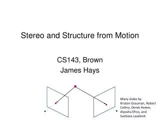
Stereoand Structure from Motion CS143, Brown James Hays Many slides by Kristen Grauman, Robert Collins, Derek Hoiem, Alyosha Efros, and Svetlana Lazebnik
Depth from disparity X (X – X’) / f = baseline / z X – X’ = (baseline*f) / z z = (baseline*f) / (X – X’) z x’ x f f baseline C’ C
Outline • Human stereopsis • Stereograms • Epipolar geometry and the epipolar constraint • Case example with parallel optical axes • General case with calibrated cameras
General case, with calibrated cameras • The two cameras need not have parallel optical axes. Vs.
Stereo correspondence constraints • Given p in left image, where can corresponding point p’ be?
Epipolar constraint Geometry of two views constrains where the corresponding pixel for some image point in the first view must occur in the second view. • It must be on the line carved out by a plane connecting the world point and optical centers.
Epipolar geometry Epipolar Line • Epipolar Plane Baseline Epipole Epipole http://www.ai.sri.com/~luong/research/Meta3DViewer/EpipolarGeo.html
Epipolar geometry: terms Why is the epipolar constraint useful? Baseline: line joining the camera centers Epipole: point of intersection of baseline with image plane Epipolar plane: plane containing baseline and world point Epipolar line: intersection of epipolar plane with the image plane All epipolar lines intersect at the epipole An epipolar plane intersects the left and right image planes in epipolar lines
Epipolar constraint This is useful because it reduces the correspondence problem to a 1D search along an epipolar line. Image from Andrew Zisserman
What do the epipolar lines look like? 1. Ol Or 2. Ol Or
Example: converging cameras Figure from Hartley & Zisserman
Example: parallel cameras Where are the epipoles? Figure from Hartley & Zisserman
Example: Forward motion What would the epipolar lines look like if the camera moves directly forward?
Example: Forward motion e’ e Epipole has same coordinates in both images. Points move along lines radiating from e: “Focus of expansion”
l • l’ • p • p’ Fundamental matrix • Let p be a point in left image, p’ in right image • Epipolar relation • p maps to epipolar line l’ • p’ maps to epipolar line l • Epipolar mapping described by a 3x3 matrix F • It follows that
Fundamental matrix • This matrix F is called • the “Essential Matrix” • when image intrinsic parameters are known • the “Fundamental Matrix” • more generally (uncalibrated case) • Can solve for F from point correspondences • Each (p, p’) pair gives one linear equation in entries of F • F has 9 entries, but really only 7 or 8 degrees of freedom. • With 8 points it is simple to solve for F, but it is also possible with 7. See Marc Pollefey’s notes for a nice tutorial
Stereo image rectification • Reproject image planes onto a common plane parallel to the line between camera centers • Pixel motion is horizontal after this transformation • Two homographies (3x3 transform), one for each input image reprojection • C. Loop and Z. Zhang. Computing Rectifying Homographies for Stereo Vision. IEEE Conf. Computer Vision and Pattern Recognition, 1999.
The correspondence problem • Epipolar geometry constrains our search, but we still have a difficult correspondence problem.
Basic stereo matching algorithm • If necessary, rectify the two stereo images to transform epipolar lines into scanlines • For each pixel x in the first image • Find corresponding epipolarscanline in the right image • Examine all pixels on the scanline and pick the best match x’ • Compute disparity x-x’ and set depth(x) = fB/(x-x’)
Correspondence search Left Right • Slide a window along the right scanline and compare contents of that window with the reference window in the left image • Matching cost: SSD or normalized correlation scanline Matching cost disparity
Correspondence search Left Right scanline SSD
Correspondence search Left Right scanline Norm. corr
Effect of window size W = 3 W = 20 • Smaller window + More detail • More noise • Larger window + Smoother disparity maps • Less detail
Failures of correspondence search Occlusions, repetition Textureless surfaces Non-Lambertian surfaces, specularities
Results with window search Data Window-based matching Ground truth
How can we improve window-based matching? • So far, matches are independent for each point • What constraints or priors can we add?
Stereo constraints/priors • Uniqueness • For any point in one image, there should be at most one matching point in the other image
Stereo constraints/priors • Uniqueness • For any point in one image, there should be at most one matching point in the other image • Ordering • Corresponding points should be in the same order in both views
Stereo constraints/priors • Uniqueness • For any point in one image, there should be at most one matching point in the other image • Ordering • Corresponding points should be in the same order in both views Ordering constraint doesn’t hold
Priors and constraints • Uniqueness • For any point in one image, there should be at most one matching point in the other image • Ordering • Corresponding points should be in the same order in both views • Smoothness • We expect disparity values to change slowly (for the most part)
Left image • Right image Scanline stereo • Try to coherently match pixels on the entire scanline • Different scanlines are still optimized independently
Left image • Right image • Right • occlusion • q • Left occlusion • t • s • p “Shortest paths” for scan-line stereo • correspondence Can be implemented with dynamic programming Ohta & Kanade ’85, Cox et al. ‘96 • Slide credit: Y. Boykov
Coherent stereo on 2D grid • Scanline stereo generates streaking artifacts • Can’t use dynamic programming to find spatially coherent disparities/ correspondences on a 2D grid
Stereo matching as energy minimization (random field interpretation) • Energy functions of this form can be minimized using graph cuts • I2 • D • I1 • W1(i) • W2(i+D(i)) • D(i) • data term • smoothness term Y. Boykov, O. Veksler, and R. Zabih, Fast Approximate Energy Minimization via Graph Cuts, PAMI 2001
Many of these constraints can be encoded in an energy function and solved using graph cuts Before Ground truth Graph cuts Y. Boykov, O. Veksler, and R. Zabih, Fast Approximate Energy Minimization via Graph Cuts, PAMI 2001 For the latest and greatest: http://www.middlebury.edu/stereo/
camera • projector Active stereo with structured light • Project “structured” light patterns onto the object • Simplifies the correspondence problem • Allows us to use only one camera • L. Zhang, B. Curless, and S. M. Seitz. Rapid Shape Acquisition Using Color Structured Light and Multi-pass Dynamic Programming.3DPVT 2002
Kinect: Structured infrared light • http://bbzippo.wordpress.com/2010/11/28/kinect-in-infrared/
Summary: Key idea: Epipolar constraint • X • X • X • x • x’ • x’ • x’ • Potential matches for x have to lie on the corresponding line l’. • Potential matches for x’ have to lie on the corresponding line l.
Summary • Epipolar geometry • Epipoles are intersection of baseline with image planes • Matching point in second image is on a line passing through its epipole • Fundamental matrix maps from a point in one image to a line (its epipolar line) in the other • Can solve for F given corresponding points (e.g., interest points) • Stereo depth estimation • Estimate disparity by finding corresponding points along scanlines • Depth is inverse to disparity
Structure from motion • Given a set of corresponding points in two or more images, compute the camera parameters and the 3D point coordinates • ? • ? • Camera 1 • ? • Camera 3 • ? • Camera 2 • R1,t1 • R3,t3 • R2,t2 • Slide credit: Noah Snavely
Structure from motion ambiguity • If we scale the entire scene by some factor k and, at the same time, scale the camera matrices by the factor of 1/k, the projections of the scene points in the image remain exactly the same: It is impossible to recover the absolute scale of the scene!