
Dynamic Branch Prediction
E N D
Presentation Transcript
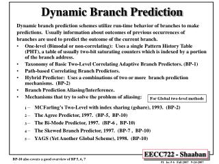
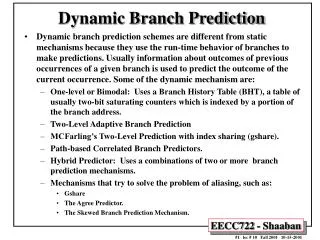
Dynamic Branch Prediction • Dynamic branch prediction schemes are different from static mechanisms because they use the run-time behavior of branches to make predictions. Usually information about outcomes of previous occurrences of a given branch is used to predict the outcome of the current occurrence. Some of the dynamic mechanism are: • One-level or Bimodal: Uses a Branch History Table (BHT), a table of usually two-bit saturating counters which is indexed by a portion of the branch address. • Two-Level Adaptive Branch Prediction • MCFarling’s Two-Level Prediction with index sharing (gshare). • Path-based Correlated Branch Predictors. • Hybrid Predictor: Uses a combinations of two or more branch prediction mechanisms. • Mechanisms that try to solve the problem of aliasing, such as: • Gshare • The Agree Predictor. • The Skewed Branch Prediction Mechanism.
Branch Target Buffer (BTB) • Effective branch prediction requires the target of the branch at an early pipeline stage. • One can use additional adders to calculate the target, as soon as the branch instruction is decoded. This would mean that one has to wait until the ID stage before the target of the branch can be fetched, taken branches would be fetched with a one-cycle penalty. • To avoid this problem one can use a Branch Target Buffer (BTB). A typical BTB is an associative memory where the addresses of branch instructions are stored together with their target addresses. • Some designs store n prediction bits as well, implementing a combined BTB and BHT. • Instructions are fetched from the target stored in the BTB in case the branch is predicted-taken. After the branch has been resolved the BTB is updated. If a branch is encountered for the first time a new entry is created once it is resolved. • Branch Target Instruction Cache (BTIC): A variation of BTB which caches the code of the branch target instruction instead of its address. This eliminates the need to fetch the target instruction from the instruction cache or from memory.
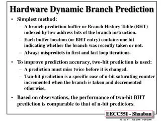
One-Level Bimodal Branch Predictors • One-level or bimodal branch prediction uses only one level of branch history. • These mechanisms usually employ a table which is indexed by lower bits of the branch address. • The table entry consists of n history bits, which form an n-bit automaton. • Smith proposed such a scheme, known as the Smith algorithm, that uses a table of two-bit saturating counters. • One rarely finds the use of more than 3 history bits in the literature. • Two variations of this mechanism: • Decode History Table: Consists of directly mapped entries. • Branch History Table (BHT): Stores the branch address as a tag. It is associative and enables one to identify the branch instruction during IF by comparing the address of an instruction with the stored branch addresses in the table.
Basic Dynamic Two-Bit Branch Prediction: Two-bit Predictor State Transition Diagram
Prediction Accuracy of A 4096-Entry Basic Dynamic Two-Bit Branch Predictor
From The Analysis of Static Branch Prediction : DLX Performance Using Canceling Delay Branches
Correlating Branches Recent branches are possibly correlated: The behavior of recently executed branches affects prediction of current branch. Example: Branch B3 is correlated with branches B1, B2. If B1, B2 are both not taken, then B3 will be taken. Using only the behavior of one branch cannot detect this behavior. SUBI R3, R1, #2 BENZ R3, L1 ; b1 (aa!=2) ADD R1, R0, R0 ; aa==0 L1: SUBI R3, R1, #2 BNEZ R3, L2 ; b2 (bb!=2) ADD R2, R0, R0 ; bb==0 L2 SUB R3, R1, R2 ; R3=aa-bb BEQZ R3, L3 ; b3 (aa==bb) B1 if (aa==2) aa=0; B2 if (bb==2) bb=0; B3 if (aa!==bb){
Two-Level Adaptive Predictors • Two-level adaptive predictors were originally proposed by Yeh and Patt (1991). • They use two levels of branch history. • The first level stored in a Branch History Register (BHR), or Table (BHT), usually a k-bit shift register. • The data in this register is used to index the second level of history, the Pattern History Table (PHT). • Yeh and Patt later identified nine variations of this mechanism depending on how branch history and pattern history is kept: per address, globally or per set, plus they give a taxonomy (1993).
A General Two-level Predictor or Path History Register (PHR)
Hardware cost of Two-level Adaptive Prediction Mechanisms • Neglecting logic cost and assuming 2-bit of pattern history for each entry. The parameters are as follows: • k is the length of the history registers, • b is the number of branches, • p is the number of sets of branches in the PHT, • s is the number of sets of branches in HRT.
Variations of global history Two-Level Adaptive Branch Prediction.
Performance of Global history schemes with different branch history lengths • The average prediction accuracy of integer (int) and floating point (fp) programs by using global history schemes. These curves are cut of when the implementation cost exceeds 512K bits.
Performance of Global history schemes with different number of pattern history tables
Variations of per-address historyTwo-Level Adaptive Branch Prediction
Performance of Per-address history schemes with different branch history lengths
Performance of Per-address history schemes with different number of pattern history tables
Variations of per-set history Two-Level Adaptive Branch Prediction
Performance of Per-set history schemes with different branch history lengths
Performance of Per-set history schemes with different number of pattern history tables
Comparison of the most effective configuration of each class of Two-Level Adaptive Branch Prediction with an implementation cost of 8K bits
Comparison of the most effective configuration of each class of Two-Level Adaptive Branch Prediction with an implementation cost of 128K bits
Correlating Two-Level Dynamic GAp Branch Predictors • Improve branch prediction by looking not only at the history of the branch in question but also at that of other branches: • Record the pattern of the m most recently executed branches as taken or not taken globally in BHR. • Use that pattern to select the proper PHT. • In general, the notation: (m,n) GAp predictor means: • Record last m branches to select between 2m PHTs. • Each table uses n-bit counters (each table entry has n bits). • Basic two-bit Bimodal BHT is then a (0,2) predictor.
GAp Predictor • The branch history is kept globally, the pattern history per branch address. (BHR) GAp (2,2) (PHTs)
Prediction Accuracy of Two-Bit Dynamic Predictors Under SPEC89 Basic Basic Correlating Two-level GAp
MCFarling's gshare Predictor • McFarling notes (1993) that using global history information might be less efficient than simply using the address of the branch instruction, especially for small predictors. • He suggests using both global history and branch address by hashing them together. He proposes using the XOR of global branch history and branch address since he expects that this value has more information than either one of its components. • This gives a more uniform distribution and usage of the PHT entries reducing interference. • The result is that this mechanism outperforms a GAp scheme by a small margin. • This mechanism seems to use substantially less hardware, since both branch and pattern history are kept globally. • The hardware cost for k history bits is k + 2 x 2k , neglecting costs for logic.
gshare Predictor Branch and pattern history are kept globally. History and branch address are XORed and the result is used to index the PHT.
Path-Based Prediction • Ravi Nair proposed (1995) to use the path leading to a conditional branch rather than the branch history in the first level to index the PHT. • The global history register of a GAp scheme is replaced by by a Path History Register, which encodes the addresses of the targets of the preceding p branches. • The path history register could be organized as a g bit shift register which encodes q bits of the last p target addresses, where g = p x q. • The hardware cost of such a mechanism is similar to that of a GAp scheme. If b branches are kept in the prediction data structure the cost is g +b x 2 x 2g . • The performance of this mechanism is similar to a comparable or better than branch history schemes for the case of no context switching. For the case that there is context switching, that is, if the processor switches between multiple processes running on the system, Nair proposes flushing the prediction data structures at regular intervals to improve accuracy. In such a scenario the mechanism performs slightly better than a comparable GAp predictor.
Hybrid or Combined Predictors • Hybrid predictors are simply combinations of other branch prediction mechanisms. • This approach takes into account that different mechanisms may perform best for different branch scenarios. • McFarling (1993) presented a number of different combinations of two branch prediction mechanisms. • He proposed to use an additional 2-bit counter array which serves to select the appropriate predictor. • One predictor is chosen for the higher two counts, the second one for the lower two counts. • If the first predictor is wrong and the second one is right the counter is decremented, if the first one is right and the second one is wrong, the counter is incremented. No changes are carried out if both predictors are correct or wrong.
MCFarling’s Combined Predictor Structure The combined predictor contains an additional counter array with 2-bit up/down saturating counters. Which serves to select the best predictor to use. Each counter keeps track of which predictor is more accurate for the branches that share that counter. Specifically, using the notation P1c and P2c to denote whether predictors P1 and P2 are correct respectively, the counter is incremented or decremented by P1c-P2c as shown below.
Branch Prediction Aliasing/Intereference • Aliasing/Intereference occurs when different branches point to the same prediction bits. • If the branch prediction mechanism is a one-level mechanism, k lower bits of the branch address are used to index the table. Two branches with the same lower k bits point to the same prediction bits. • Similarly, in a PAg two-level scheme, the pattern history is indexed by the contents of history registers. If two branches have the same k history bits they will point to the same predictor entry in PHT. • Three different cases of aliasing: • Constructive aliasing improves the prediction accuracy, • Destructive aliasing decreases the prediction accuracy, and • Harmless aliasing does not change the prediction accuracy. • An alternative definition of aliasing applies the "three-C" model of cache misses to aliasing. Where aliasing is classified as three cases: • Compulsory aliasing occurs when a branch substream is encountered for the first time. • Capacity aliasing is due to the programs working set being too large to fit into the prediction data structures. Increasing the size of the data structures can reduce this effect. • Conflict aliasing occurs when two concurrently-active branch substreams map to the same predictor-table entry.
Interference Reduction Prediction Schemes • Gshare, 1993. • The Agree Predictor, 1997. • The Bi-Mode Predictor, 1997. • The Skewed Branch Predictor, 1997. • The Filter Mechanism, 1996). • YAGS (Yet Another Global Scheme), 1998.
The Agree Predictor • The Agree Predictor is a scheme that tries to deal with the problem of aliasing, proposed by Sprangle, Chappell, Alsup and Patt • They distinguish three approaches to counteract the interference problem: • Increasing predictor size to cause conflicting branches to map to dierent table locations. • Selecting a history table indexing function that distributes history states evenly among available counters. • Separating different classes of branches so that they do not use the same prediction scheme. • The Agree predictor converts negative interference into positive or neutral interference by attaching a biasing bit to each branch, for instance in the BTB or instruction cache, which predicts the most likely outcome of the branch. • The 2-bit counters of the branch prediction now predict whether or not the biasing bit is correct or not. The counters are updated after the branch has been resolved, agreement with the biasing bit leads to incrementing the counters, if there is no agreement the counter is decremented. The biasing bit could be determined by the direction the branch takes at the first occurrence.
The Agree Predictor • The hardware cost of this mechanism is that of the two-level adaptive mechanism it is based on, plus one bit per BTB entry or entry in the instruction cache. • Simulations show that this scheme outperforms other mechanisms, especially for smaller predictor sizes, because there is more contention than in bigger predictors.
The Bi-Mode Predictor • The Bi-Mode Predictor. The bi-mode predictor tries to replace destructive aliasing with neutral aliasing • It splits the PHT table into even parts. One of the parts is the choice PHT, which is just a bimodal predictor with a slight change in the updating procedure. • The other two parts are direction PHTs; one is a “taken” direction PHT and the other is a “not taken” direction PHT. The direction PHTs are indexed by the branch address XORed with the global history. • When a branch is present, its address points to the choice PHT entry which in turn chooses between the “taken” direction PHT and the “not taken” direction PHT. The prediction of the direction PHT chosen by the choice PHT serves as the prediction. Only the direction PHT chosen by the choice PHT is updated. • As a result of this scheme, branches which are biased to be taken will have their predictions in the “taken” direction PHT, and branches which are biased not to be taken will have their predictions in the “not taken” direction PHT. So at any given time most of the information stored in the “taken” direction PHT entries is “taken” and any aliasing is more likely not to be destructive. • In contrast to the agree predictor, if the bias is incorrectly chosen the first time the branch is introduced to the BTB, it is not bound to stay that way while the branch is in the BTB and as a result pollute the direction PHTs. • However, it does not solve the aliasing problem between instances of a branch which do not agree with the bias and instances which do.
The Skewed Branch Predictor • The skewed branch predictor is based on the observation that most aliasing occurs not because the size of the PHT is too small, but because of a lack of associativity in the PHT (the major contributor to aliasing is conflict aliasing and not capacity aliasing). • The best way to deal with conflict aliasing is to make the PHT set-associative, but this requires tags and is not cost-effective. • Instead, the skewed predictor emulates associativity using a special skewing function. • The skewed branch predictor splits the PHT into three even banks and hashes each index to a 2-bit saturating counter in each bank using a unique hashing function per bank (f1, f2 and f3). • The prediction is made according to a majority vote among the three banks. If the prediction is wrong all three banks are updated. If the prediction is correct, only the banks that made a correct prediction will be updated (partial updating). • The skewing function should have inter-bank dispersion. This is needed to make sure that if a branch is aliased in one bank it will not be aliased in the other two banks, so the majority vote will produce an unaliased prediction. • The reasoning behind partial updating is that if a bank gives a misprediction while the other two give correct predictions, the bank with the misprediction probably holds information which belongs to a different branch. In order to maintain the accuracy of the other branch, this bank is not updated. • The skewed branch predictor tries to eliminate all aliasing instances and therefore all destructive aliasing. Unlike the other methods, it tries to eliminate destructive aliasing between branch instances which obey the bias and those which do not.
Yet Another Global Scheme (YAGS) • As done in the agree and bi-mode, YAGS reduces aliasing by splitting the PHT into two branch streams corresponding to biases of “taken” and “not taken”. • However, as in the skewed branch predictor, we do not want to neglect aliasing between biased branches and their instances which do not comply with the bias. • The motivation behind YAGS is the observation that for each branch we need to store its bias and the instances when it does not agree with it. • A bimodal predictor is used to store the bias, as the choice predictor does in the bi-mode scheme. All we need to store in the direction PHTs are the instances when the branch does not comply with its bias. • To identify those instances in the direction PHTs small tags (6-8 bits) are added to each entry, referring to them (PHTs) now as direction caches. These tags store the least significant bits of the branch address and they virtually eliminate aliasing between two consecutive branches. • When a branch occurs in the instruction stream, the choice PHT is accessed. If the choice PHT indicated “taken,” the “not taken” cache is accessed to check if it is a special case where the prediction does not agree with the bias. If there is a miss in the “not taken” cache, the choice PHT is used • as a prediction. If there is a hit in the “not taken” cache it supplies the prediction. A similar set of actions is taken if the choice PHT indicates “not taken,” but this time the check is done in the “taken” cache. • The choice PHT is addressed and updated as in the bi-mode choice PHT. The “not taken” cache is updated if a prediction from it was used. It is also updated if the choice PHT is indicating “taken” and the branch outcome was “not taken.” The same happens with the “taken” cache. • Aliasing for instances of a branch which do not agree with the branch’s bias is reduced by making the direction caches set-associative: • LRU replacement is used policy with one exception: an entry in the “taken” cache which indicates “not taken” will be replaced first to avoid redundant information. If an entry in the “taken” cache indicates “not taken,” this information is already in the choice PHT and therefore is redundant and can be replaced.