Download

1 / 40
400 likes | 553 Views
Lecture 4: Topic #1 Extent (How Much) Decisions Marginal Revenue, Costs (Average and Marginal) Remember, We always think on the MARGIN. Lecture 4: Topic 1 – Summary of main points. Do not confuse average and marginal costs.

E N D
Lecture 4: Topic #1Extent (How Much) DecisionsMarginal Revenue, Costs (Average and Marginal)Remember, We always think on the MARGIN
Lecture 4: Topic 1 – Summary of main points • Do not confuse average and marginal costs. • Average cost (AC) is total cost (fixed and variable) divided by total units produced. • Average cost is irrelevant to an extent decision. • Marginal cost (MC) is the additional cost incurred by producing and selling one more unit.
Lecture 4: Topic #1 – Summary • Marginal revenue (MR) is the additional revenue gained from selling one more unit. • Sell more if MR > MC; sell less if MR < MC. If MR = MC, you are selling the right amount (maximizing profit). • The relevant costs and benefits of an extent decision are marginal costs and marginal revenue. If the marginal revenue of an activity is larger than the marginal cost, then do more of it. • An incentive compensation scheme that increases marginal revenue or reduces marginal cost will increase effort. Fixed fees have no effects on effort. • A good incentive compensation scheme links pay to performance measures that reflect effort.
Introductory anecdote: US Financial Crisis • The financial crisis began in the subprime housing market, where government policies encouraged lenders to extend credit to low-income borrowers (by lowering lending standards) • Concurrently mortgages were being packaged into securities and sold to investors. • If the risk had been recognized investor demand would have been low, but rating agencies were too liberal with AAA ratings, increasing demand for loans. • The result? A credit “bubble” • How did this lending crisis arise?
Background: Average cost • Definition: Average cost is simply the total cost of production divided by the number of units produced. AC = TC/Q • Average costs often decrease as quantity increases due to presence of fixed costs • AC = (VC + FC)/Q • FC does not change as Q increases • Average costs are not relevant to extent decisions
Background: Marginal cost • Marginal cost is the cost to make and sell one additional unit of output. MC = TCQ+1 – TCQ. • Marginal cost is often lower than average cost (due to falling average costs) but not always. • Marginal costs are what matter in extent decisions
Extent (how much?) decisions • Definition: Marginal cost (MC) is the additional cost required to produce and sell one more unit. • Definition: Marginal revenue (MR) is the additional revenue gained from producing and selling one more unit. • If the benefits of selling another unit (MR) are bigger than the costs (MC), then sell another unit. • So, produce more when MR>MC; less when MR<MC. Profits are maximized when MR=MC.
Extent decisions (cont.) • Examples of extent decisions • Should you change the level of advertising? • Should you increase the quality of service? • Is your staff big enough, or too big? • How many parking spaces should you lease? • Marginal analysis answers these questions • This analysis tells you direction of change but not the distance. • You can only measure MR and MC at the current level of output – make a change and re-measure
Extent decision example • Discussion: How much advertising? • A $50,000 increase in the TV ad budget brings in 1,000 new customers • Estimated MCTV is $50 (the cost to get one more customer) • $50,000 / 1,000 = $50 • If the marginal revenue generated by this customer is greater than $50, do more advertising.
Extent decision example (cont.) • Even if we do not know the marginal revenue, we can still use marginal analysis to make extent decisions • Compare TV advertising to telephone solicitation • Say you recently cut telephone budget by $10,000 and lost 100 customers • Estimated MCPH = $100= ($10,000 / 100) • So, to get one more customer costs $50 for TV and $100 for phone • MCPH > MCTV so shift ad dollars from phone to TV • Advice: make changes one-at-a-time to gather valuable information about marginal effectiveness of each medium.
Another example • SAH=“Standard Absorbed Hours” a measure of textile factory output • Allows managers to compare factories making different items, e.g. t-shirt = 1 SAH while dress=3 SAH • Suppose Factory A has costs of $30 per SAH while Factory B has cost of $20 per SAH. How can you profitably use this information? • The decision seems simple, but • Make sure you are not including fixed costs in the analysis • Marginal costs matter, not average costs! • If the $20 and $30 rates are good MC proxies, shift some production from Factory A to Factory B
Effort is an extent decision • Discussion: Royalty rates vs. fixed fee contracts • You receive two bids to harvest 100 trees on your land • $150/tree or $15,000 for the right to harvest all the trees. • On your tract there are pines (worth $200) and fir (worth $100) • Which offer should you accept? • Discussion: Sales Commissions • Expected sales level: 100 units @ $10,000/unit=$1M • Option 1: 10% commission • Option 2: 5% commission + $50,000 salary
Tie pay to performance • A consulting firm COO received a flat salary of $75,000 • After learning about the benefits of incentive pay in class, the CEO changed COO compensation to $50K + (1/3)* (Profits-$150K) • Profits increased 74% to $1.2 M • Compensation increased $75K $177K • Discussion: what are the disadvantages to incentive pay?
Alternate intro anecdote • American Express offers a Platinum Card to affluent customers • In 2001, there were approximately 2,000 Platinum cardholders in the Japanese market. Numbers had been limited to ensure high quality customer service • With customer service technology advances, company considered expanding number of card holders • How many more should be added? • As more members are acquired, average spending per card member decreases because the financial threshold for membership is lowered • Costs of customer service rise for each additional member added, and growing beyond a certain point would require building and operating an additional call center • After analyzing the costs and benefits, American Express realized that it should expand its offering to only 15,000 more Platinum Card members • We call this an “extent” decision, because the company needed to decide “how many” platinum cards to provide. In this lecture, we show you how to make profitable extent decisions.
Summary of main points • Aggregate demand or market demand is the total number of units that will be purchased by a group of consumers at a given price. • Pricing is an extent decision. Reduce price (increase quantity) if MR > MC. Increase price (reduce quantity) if MR < MC. The optimal price is where MR = MC. • Price elasticity of demand, e = (% change in quantity demanded) ÷ (% change in price) • Estimated price elasticity = [(Q1 - Q2)/(Q1 + Q2)] ÷ [(P1 - P2)/(P1 + P2)] is used to estimate demand from a price and quantity change. • If |e| > 1, demand is elastic; if |e| < 1, demand is inelastic. • %ΔRevenue ≈ %ΔPrice + %ΔQuantity • Elastic Demand (|e| > 1): Quantity changes more than price. • Inelastic Demand (|e| < 1): Quantity changes less than price.
Summary (cont.) • MR > MC implies that (P - MC)/P > 1/|e|; in words, if the actual markup is bigger than the desired markup, reduce price • Equivalently, sell more • Four factors make demand more elastic: • Products with close substitutes (or distant complements) have more elastic demand. • Demand for brands is more elastic than industry demand. • In the long run, demand becomes more elastic. • As price increases, demand becomes more elastic. • Income elasticity, cross-price elasticity, and advertising elasticity are measures of how changes in these other factors affect demand. • It is possible to use elasticity to forecast changes in demand: %ΔQuantity ≈ (factor elasticity)*(%ΔFactor). • Stay-even analysis can be used to determine the volume required to offset a change in costs or prices.
Introductory anecdote: Gas prices • US: From early 2007 to mid 2008 gas prices rose in the US. • Gas prices caused people to find alternate methods of work and travel to avoid using gas. • Some farms began using mules instead of tractors • India: In Rajasthan, the rising gas prices caused many farmers to switch from tractors to camels on farms. • As oil prices rose, demand for camels increased. • Prices for camels tripled over a two-year period. • A US company, NNS, that produces potash fertilizer experienced an increase in input costs due to their use of petrochemicals. • NNS doubled the price of the generic fertilizer, and priced it’s branded fertilizer at a 35% premium above the generic price. • Costs increased rapidly over the first two quarters combined with NNS’s policy of quarterly price revision led to stockouts and a price that ended up being 25% below the generic – NNS could have earned $13 million but failed to maintain their premium
Background: consumer surplus and demand curves • First Law of Demand - consumers demand (purchase) more as price falls, assuming other factors are held constant. • Consumers make consumption decisions using marginal analysis, consume more if marginal value > price • But, the marginal value of consuming each subsequent unit diminishes the more you consume. • Consumer surplus = value to consumer - price paid • Definition: Demand curves are functions that relate the price of a product to the quantity demanded by consumers
Background: consumer surplus and demand curves (cont.) • Hot dog consumer • Values first dog at $5, next at $4 . . . fifth at $1 • Note that if hot dogs price is $3, consumer will purchase 3 hot dogs
Background: aggregate demand • Aggregate Demand: the buying behavior of a group of consumers; a total of all the individual demand curves. • To construct demand, sort by value. • Discussion: Why do aggregate demand curves slope downward? • Role of heterogeneity? • How to estimate?
Pricing trade-off • Pricing is an extent decision • Profit= Revenue - Cost • Demand curves turn pricing decisions into quantity decisions: “what price should I charge?” is equivalent to “how much should I sell?” • Fundamental tradeoff: • Lower price sell more, but earn less on each unit sold • Higher price sell less, but earn more on each unit sold • Tradeoff created by downward sloping demand
Marginal analysis of pricing • Marginal analysis finds the profit increasing solution to the pricing tradeoff. • It tells you only whether to raise or lower price, not . • Definition: marginal revenue (MR) is change in total revenue from selling extra unit. • If MR>0, then total revenue will increase if you sell one more. • If MR>MC, then total profits will increase if you sell one more. • Proposition: Profits are maximized when MR = MC
Example: finding the optimal price • Start from the top • If MR > MC, reduce price (sell one more unit) • Continue until the next price cut (additional sale) until MR<MC
How do we estimate MR? • Price elasticity is a factor in calculating MR. • Definition: price elasticity of demand (e) • (%change in quantity demanded) (%change in price) • If |e| is less than one, demand is said to be inelastic. • If |e| is greater than one, demand is said to be elastic.
Estimating elasticities • Definition: Arc (price) elasticity= [(q1-q2)/(q1+q2)] [(p1-p2)/(p1+p2)]. • Discussion: Why, when price changes from $10 to $8, does quantity changes from 1 to 2? • Example:On a promotion week for Vlasic, the price of Vlasic pickles dropped by 25% and quantity increased by 300%. • Is the price elasticity of demand -12? • HINT: could something other than price be changing?
Estimating elasticities (cont.) • 3-Liter Coke Promotion (Instituted to meet Wal-Mart promotion) • Compute price elasticity of 3 liter coke; cross price elasticity of 2 liter coke with respect to 3 liter price;
Intuition: MR and price elasticity • Revenue and price elasticity are related. • %Rev ≈%P + %Q • Elasticity tells you the size of |%P| relative to |%Q| • If demand is elastic • If P↑ then Rev↓ • If P↓ then Rev↑ • If demand is inelastic • If P↑ then Rev↑ • If P↓ then Rev↓ • Discussion: In 1980, Marion Barry, mayor of the District of Columbia, raised the sales tax on gasoline sold in the District by 6%. What happened to gas sales and availability of gas? Why?
Formula: elasticity and MR • Proposition: MR = P(1-1/|e|) • If |e|>1, MR>0. • If |e|<1, MR<0. • Discussion: If demand for Nike sneakers is inelastic, should Nike raise or lower price? • Discussion: If demand for Nike sneakers is elastic, should Nike raise or lower price?
Elasticity and pricing • MR>MC is equivalent to • P(1-1/|e|)>MC • P>MC/(1-1/|e|) • (P-MC)/P>1/|e| • Discussion: e= –2, p=$10, mc= $8, should you raise prices? • Discussion: mark-up of 3-liter Coke is 2.7%. Should you raise the price? • Discussion: Sales people MR>0 vs. marketing MR>MC.
What makes demand more elastic? • Products with close substitutes have elastic demand. • Demand for an individual brand is more elastic than industry aggregate demand. • Products with many complements have less elastic demand.
Describing demand with price elasticity • First law of demand: e < 0 ( as price goes up, quantity goes down). • Discussion: Do all demand curves slope downward? • Second law of demand: in the long run, |e| increases. • Discussion: Give an example of the second law of demand.
Describing demand (cont.) • Third law of demand: as price increases, demand curves become more price elastic, |e| increases. • Discussion: Give an example of the third law of demand.
Other elasticities • Definition: income elasticity measures the change in demand arising from a change in income • (%change in quantity demanded) (%change in income) • Inferior (neg.) vs. normal (pos). • Definition: cross-price elasticity of good one with respect to the price of good two • (%change in quantity of good one) (%change in price of good two) • Substitute (pos.) vs. complement (neg.). • Definition: advertising elasticity; a change in demand arising form a change in advertising • (%change in quantity) (%change in advertising) . • Discussion: The income elasticity of demand for WSJ is 0.50. Real income grew by 3.5% in the United States. • Estimate WSJ demand
Stay-even analysis • Stay-even analysis tells you how many sales you need when changing price to maintain the same profit level • Q1 = Q0*(P0-VC0)/(P1-VC0) • When combined with information about the elasticity of demand, the analysis gives a quick answer to the question of whether or not changing price makes sense. • To see the effect of a variety of potential price changes, we can draw a stay-even curve that shows the required quantities at a variety of price levels.
Stay-even curve example • Note that if demand is elastic, price cuts increase revenue • When demand is inelastic, price increases will increase revenue
Extra: quick and dirty estimators • Linear Demand Curve Formula, e= p / (pmax-p) • Discussion: How high would the price of the brand have to go before you would switch to another brand of running shoes? • Discussion: How high would the price of all running shoes have to go before you should switch to a different type of shoe?
Extra: market share formula • Proposition: The individual brand demand elasticity is approximately equal to the industry elasticity divided by the brand share. • Discussion: Suppose that the elasticity of demand for running shoes is –0.4 and the market share of a Saucony brand running shoe is 20%. What is the price elasticity of demand for Saucony running shoes? • Proposition: Demand for aggregate categories is less-elastic than demand for the individual brands in aggregate.
Alternate introductory anecdote • In 1994, the peso devalued by 40% in Mexico • Interest rates and unemployment shot up • Overall economy slowed dramatically and consumer income fell • Concurrently, demand for Sara Lee hot dogs declined • This surprised managers because they thought demand would hold steady, or even increase, since hot dogs were more of a consumer staple than a luxury item. • Surveys revealed the decline was mostly confined to premium hot dogs • And, consumers were using creative substitutes • Lower priced brands did take off but were priced too low. • Failure to understand demand and to price accordingly was costly