CORRELATION COEFFICIENT LINEAR REGRESSION معامل الارتباط و الانحدار

1. CORRELATION COEFFICIENTLINEAR REGRESSIONمعامل الارتباط و الانحدار By: Amani Albraikan

2. Pearson r • Spearman rho

3. Factors Affecting Correlation • Linearity • Range restrictions • Outliers • Beware of spurious correlations….take care in interpretation • High positive correlation between a country’s infant mortality rate and the no. of physicians per 100,000 population

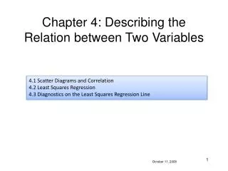
4. General Overview of Correlational Analysis • The purpose is to measure the strength of a linear relationship between 2 variables. • A correlation coefficient does not ensure “causation” (i.e. a change in X causes a change in Y) • X is typically the Input, Measured, or Independent variable. • Y is typically the Output, Predicted, or Dependent variable. • If, as X increases, there is a predictable shift in the values of Y, a correlation exists.

5. General Properties of Correlation Coefficients • Values can range between +1 and -1 • The value of the correlation coefficient represents the scatter of points on a scatterplot • You should be able to look at a scatterplot and estimate what the correlation would be • You should be able to look at a correlation coefficient and visualize the scatterplot

6. Perfect Linear Correlation • Occurs when all the points in a scatterplot fall exactly along a straight line.

7. Positive CorrelationDirect Relationship • As the value of X increases, the value of Y also increases • Larger values of X tend to be paired with larger values of Y (and consequently, smaller values of X and Y tend to be paired)

8. Negative CorrelationInverse Relationship • As the value of X increases, the value of Y decreases • Small values of X tend to be paired with large value of Y (and vice versa).

9. Non-Linear Correlation • As the value of X increases, the value of Y changes in a non-linear manner

10. No Correlation • As the value of X changes, Y does not change in a predictable manner. • Large values of X seem just as likely to be paired with small values of Y as with large values of Y

11. Interpretation • Depends on what the purpose of the study is… but here is a “general guideline”... • Value = magnitude of the relationship • Sign = direction of the relationship

12. Some of the manyTypes of Correlation Coefficients(there are lot’s more…)

13. Some of the manyTypes of Correlation Coefficients(there are lot’s more…. these are the ones we willfocus on this semester) Included in SPSS “Bivariate Correlation” procedure

14. The Pearson Product-Moment Correlation (r) • Named after Karl Pearson (1857-1936) • Both X and Y measured at the Interval/Ratio level • Most widely used coefficient in the literature

15. The Pearson Product-Moment Correlation (r) • A measure of the extent to which paired scores occupy the same or opposite positions within their own distributions From: Pagano (1994)

16. Computing Pearson r Hand Calculation

17. Interpretation • r = 0.73 : p = .161 The researchers found a moderate, but not-significant, relationship between X and Y

18. Interpretation • r = 0.73 : p = .000 The researchers found a significant moderate relationship between X and Y

19. Calculation of Pearson’s Correlation Coefficient r

20. Pearson’s Correlation Coefficient r Source data (p.202): Spice sales vs. shelf space

21. CORRELATION COEFFICIENT The point is that neither the first path nor the second one do withstand the numerical competition with the so called the Pearson product moment correlation coefficient despite its complex and apparently non attractive clothes as they are seen below:

22. CORRELATION COEFFICIENT Choosing the significance level atwe shall find that for 18 d.f.which allows us to reject null hypotheses that the correlation coefficient is equal to zero even at such highsignificance level. From the other side it is reasonable to add that the correlation coefficient measures the strength of the linear relation between both considered variables. In practice it isconvenient to use for statistical inferences indications shown below: Our further considerations will be related to linear regression in order to switch on the same problem but from some what different attitude.

23. The Pearson Product-Moment Correlation Coefficient • The relationship between IQ scores and grade point average? (N=12 uni students)

25. Example Serotonin Levels and Aggression in Rhesus Monkeys

26. r =1

27. r = 0.95

28. r = 0.7

29. r = 0.4

30. r = -0.4

31. r = -0.7

32. r = -0.8

33. r = -0.95

34. r = -1

35. High Groupr = 0.67 HIGH

36. Here’s another problem with interpreting Correlation Coefficients that you should watch out for….. All data combined r = +0.89 Men r = -0.21 Women r = +0.22

37. Reporting a set of Correlation Coefficients in a table Lower triangular correlation matrix. Values are not repeated. There is also an upper triangular matrix! Complete correlation matrix. Notice redundancy.

38. Spearman Rho (rs) • Named after Charles E. Spearman (1863-1945) • Assumptions: • Data consist of a random sample of n pairs of numeric or non-numeric observations that can be ranked. • Each pair of observations represents two measurement taken on the same object or individual. Photo from: http://www.york.ac.uk/depts/maths/histstat/people/sources.htm

39. Why choose Spearman rhoinstead of a Pearson r? • Both X and Y are measured at the ordinal level • Sample size is small • X and Y are measured at the interval/ratio level, but are not normally distributed (e.g. are severely skewed) • X and Y do not follow a bivariate normal distribution

42. Spearman’s Rank Correlation Coefficient D = the difference between the ranks of corresponding values of x and y n= the number of pairs of values

43. Spearman’s Rank Correlation Coefficient (example)

44. Interpretation of Correlation • Issue of Causality • - The existence of a correlation between two variables does not imply • causality • - It is possible that there were other confounding variables responsible for • the observed correlation, either in whole or in part • Description • - Correlation analysis does serve a data reduction descriptive function to • understand key variables • Prediction • - The descriptive power of correlation analysis has its potential for • prediction information • Common variance • - The square of the correlation coefficient between two variables, , • indicates that the proportion of variance in one of the variables • explained the variance of the other variable.

45. Linear Correlation and Linear Regression - Closely Linked • Linear correlation refers to the presence of a linear relationship between two variables ie a relationship that can be expressed as a straight line • Linear regression refers to the set of procedures by which we actually establish that particular straight line, which can then be used to predict a subject’s score on one of the variables from knowledge of the subject’s score on the other variable

46. To draw the regression line, choose two convenient values of X (often near the extremes of the X values to ensure greater accuracy)and substitute them in the formula to obtain the corresponding Y values, and then plot these points and join with a straight line • With the regression equation, we now have a means by which to predict a score on one variable given the information (score) of another variable • E.g. SAT score and collegiate GPA

47. What to do with OutliersYou are stuck with them unless….. • Check to see if there has been a data entry error. If so, fix the data. • Check to see if these values are plausible. Is this score within the minimum and maximum score possible? If values are impossible, delete the data. Report how many scores were deleted. • Examine other variables for these subjects to see if you can find an explanation for these scores being so different from the rest. You might be able to delete them if your reasoning is sound.