Download
1 / 17
170 likes | 436 Views
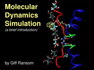
Homayoun Valafar Department of Computer Science and Engineering, USC. Introduction to Molecular Dynamics. History of Protein Motion. Proteins were anticipated (in 1950s) to be the molecules of inheritance.

E N D
Homayoun Valafar Department of Computer Science and Engineering, USC Introduction to Molecular Dynamics
CSCE 769 History of Protein Motion • Proteins were anticipated (in 1950s) to be the molecules of inheritance. • In 1958, John Kendrew and associates successfully determined the structure of myoglobin. • John Kendrew shared the 1962 Nobel Prize in chemistry with Max Perutz for his characterization of Myoglobin. • The structure was scrutinized until recently (2000). • Access to the embedded heme group was hindered. • Crystal structure shattered upon exposure to air. • Should have much more affinity to CO than O2.
CSCE 769 Brownian Motion • In 1827 the botanist Robert Brown observed the motion of plant spores floating in water and moving randomly • The explanation for this was already thought to be the random motion of molecules "hitting" the spores • The first satisfactory theoretical treatment of the Brownian motion was made by Albert Einstein in 1905 • Einstein's theory enabled significant statistical predictions about the motion of particles that are randomly distributed in a fluid • Stock market behavior
CSCE 769 Why the Blue Sky? Tyndall Effect • In 1859, John Tyndall passed a beam of white light through a clear container of water in which small, invisible particles were suspended • From the side it looked blue, but directly it looked orange. • Molecules in the air (O, N, C, Ar) exhibit Brownian motion. • Brownian motion scatters blue light • This means that white sunlight has its blue components scattered to the side while its red components keep traveling straight. White sunlight bathes the atmosphere of the earth. The sky is blue because molecules in the air scatter blue to your eyes more than they scatter red.
Maxwell-Boltzmann Distribution • Potential energy of an object with mass m raised to the height of h: • In the presence of gravitational field the concentration of gas molecules is not the same at various points of the space. • Likelihood of finding a molecule in height h is dictated by the M-B distribution. • k is the Boltzman constant (1.380×10⁻²³J/K) • T is temperature in degrees of Kelvin CSCE 769
Discrete Energy States • Bohr atomic model • Electrons can exist in discrete orbits. • Total number of entities in energy level i is dictated by MB-distribution: CSCE 769
CSCE 769 Metropolis Monte Carlo (SA) • Start at S0, E0 and T0 • Loop 1: Make a transition to S1, E1 • Accept S1 as the new state if E1 < E0 • If E1 > E0 then • Accept S1 as the new state with a probability of: • Reject S1 as the new state with a probability of: • Repeat Loop 1 N times: • Reduce temperature and repeat loop 1
CSCE 769 Contribution of Simulated Annealing Simulated annealing helps to escape from the local minima.
CSCE 769 MD Simulation with XPLOR-NIH • Initial velocities can be assigned to each atom • Using uniformly random velocities • Maxwell: • Xplor statement: • set seed=432324368 end • vector do (vx=maxwell(4000.)) ( all ) • vector do (vy=maxwell(4000.)) ( all ) • vector do (vz=maxwell(4000.)) ( all ) • Perform MD: • dynamics verlet • nstep=1000 timestep=0.001 iasvel=current • firsttemperature=300 nprint=25 end
CSCE 769 set seed=432324368 end vector do (vx=maxwell(4000.)) ( all ) vector do (vy=maxwell(4000.)) ( all ) vector do (vz=maxwell(4000.)) ( all ) evaluate ($1=4000) while ($1 > 300.0) loop main dynamics verlet timestep=0.0005 nstep=50 iasvel=current nprint=5 iprfrq=0 tcoupling=true tbath=$1 end evaluate ($1=$1-25) end loop main SA with XPLOR-NIH • Temperature needs to reduce over time. • Define the following two terms • First temperature. • Bath temperature. • Temperature can be coupled to the bath temperature and reduce over time.
Homayoun Valafar Department of Computer Science and Engineering, USC MD Simulation Part II
Newton's Laws of Motion • Newton's laws are the corner stones of the classical physics • Newton's First Law (law of inertia): • If the vector sum of all forces on an object sum up to zero, then the velocity and trajectory of that object will remain unchanged • Newton's Second Law: • Acceleration of an object is proportional to the sum of forces applied to that object • Newton's Third Law: • For every action there is an equal and opposite reaction
Laws of Thermodynamics • Laws of thermodynamics describe the transport of heat and work in thermodynamic processes • They are mostly concerned with closed systems • First Law (conservation of energy): • Energy can neither be created nor destroyed. It can only change forms. • Second Law: • Energy systems have a tendency to increase their entropy (measure of disorder) rather than decrease it. • Third Law: • As temperature approaches absolute zero, the entropy of a system approaches a constant minimum.
Basics of MD Simulation V0 FAngle FAngle FBond
Assignment of Initial Velocities in MDS • Xplor-NIH provides the following three methods of assigning initial velocities: • Blotzman-Maxwell distribution • IASVel = MAXWell • Uniform distribution • IASVel=UNIForm • Current velocities stored in vectors Vx, Vy and Vz • IASVel= CURRent set seed=432324368 end vector do (vx=maxwell(4000.)) ( all ) vector do (vy=maxwell(4000.)) ( all ) vector do (vz=maxwell(4000.)) ( all )
Role of Temperature in MD Simulations • Temperature has an impact on the initial and therefore the intermediate velocities • Xplor-NIH allows three methods of controlling temperature • We will only use velocity rescaling • IEQFrq= frequency of the velocity rescaling If ISCVel = 0 If ISCVel = 1
Demonstration • NAMD based MD simulation • Examine and understand with Xplor-NIH • MDS.BM.inp • MDS.FixedV.inp