Download
1 / 71
710 likes | 880 Views
Millimetre Astronomy. John Storey. September 28, 2001. Millimetre Astronomy. Introduction Molecular lines Science overview Toward the future. Millimetre Astronomy. Introduction Molecular lines Science overview Toward the future. At 100 GHz ( l = 3 mm):.

E N D
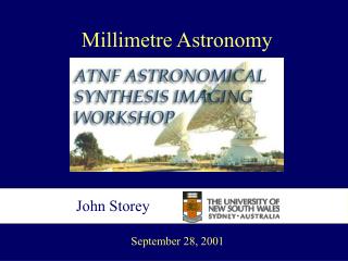
Millimetre Astronomy John Storey September 28, 2001
Millimetre Astronomy Introduction Molecular lines Science overview Toward the future
Millimetre Astronomy Introduction Molecular lines Science overview Toward the future
At 100 GHz (l = 3 mm): E = hu/q = 4 x 10⁻⁴ eV T = hu/k = 5 K This tells us what kind of phenomena we will be dealing with. But first, a few words about the earth’s atmosphere...
Trace gases Argon 0.002% 0.93% Carbon dioxide Oxygen 0.033% 21% Composition of dry air Nitrogen 78% Trace gases, (parts per million) NB: “Real” air also contains 0 ~ 5% water vapour. J.W.V. Storey, 2000
The distance from here to the stratosphere is roughly the same as the distance from Epping to the Sydney Opera House. http://liftoff.msfc.nasa.gov/
Mostly water vapour Molecular oxygen http://maisel.as.arizona.edu
12-metre, Kitt Peak, Arizona http://kp12m.as.arizona.edu/
High accuracy surface Small subreflector SEST Swedish/European Submillimetre Telescope, Chile No kangaroos http://www.ls.eso.org/
A new definition of“support astronomer”. http://www.ls.eso.org/
Nobeyama, Japan http://www.nro.nao.ac.jp/
IRAM Plateau de Bure Pico de Velata http://iram.fr/
IRAM, Pico Veleta, Spain http://www.iram.es/
IRAM, Plateau de Bure, France http://iram.fr/
BIMA—the Berkeley/Illinois/Maryland Array, Hat Creek, California. http://bima.astro.umd.edu/
Owens Valley Radio Observatory, California http://www.ovro.caltech.edu/
Mopra The mm upgrade and operation of Mopra Observatory is a collaboration between UNSW and ATNF. http://www.atnf.csiro.au
The world’s newest mm array, Narrabri, Australia. http://www.atnf.csiro.au
Millimetre Astronomy Introduction Molecular lines Science overview Toward the future
For a linear molecule such as carbon monoxide: re O m2 C Moment of inertia = I = m1m2.re2/(m1 + m2) m1 Angular momentum = Iw = 2puI
Let’s say the angular momentum, 2puI, is quantised in units of h/2p. re O m2 C Then 2puI = Jh/2p, where J = 0, 1, 2 ... m1 \u = Jh/4p2I = 2BJ, where B = h/8p2I andB is the rotational constant.
So, we have u = 2BJ. The energy levels must be given by E(J) = BJ(J+1) re O m2 C For 12C16O: B = 57.9 GHz, and we can derive re = 0.1128 nm. m1
Energy levels and spectrum of a well-behaved linear molecule. From Gordy and Cook (1970)
We call this the rigid rotor approximation. In fact, the bond between the atoms is more like a little spring, leading to centrifugal distortion. We let EJ = BJ(J + 1) - DJ2(J + 1)2, From which uJ + 1 -> J = 2BJ - 4DJ3, where D is the centrifugal distortion constant.
This simple analysis works for (almost) all linear molecules, such as HCN, HNC, HC0+, HCCCCCCCCCCCN, etc. We’ll explain the “almost” in a bit...
GHz J J J J J
GHz J J J J J J
The bigger the molecule, the larger the partition function. That is to say, at any given temperature the molecules can be distributed over a larger number of available energy levels. For any given molecule, increasing the temperature will increase the population in higher lying states, while decreasing that in the lower.
Line Intensities (linear molecules) Only certain transitions are permitted. For dipole-allowed transitions they are those with DJ = ±1. We have Aijau3|mij|2, Where Aij is the dipole moment matrix element connecting the two states i and j, and depends on the molecule’s dipole moment, m. For CO, m = 0.10 D. For HCN, m = 3.00 D.
Line Intensities (linear molecules) For CO, m = 0.10 D. For HCN, m = 3.00 D. The A coefficient for the J = 1 -> 0 transition of HCN is therefore ~1000 times that of CO. Molecules such as N2 and H2 have no dipole moment and thus have no dipole-allowed transitions.
Line Intensities (any molecule) The observed emission line intensity depends on the A coefficient, Aij , and the column density of molecules in the upper state, which in turn depends on: • The column density of H2 • The molecular abundance relative to H2 • The molecular partition function • The temperature of the gas • The density of the gas. (Assuming, of course, that the line is optically thin. If it is optically thick, the intensity depends only on the gas temperature.)
For 2- and 3- dimensional molecules, such as methyl cyanide (CH3CN), x z we identify the three principal axes and then define A, B, C as A = h/8p2IA etc., with A > B > C. y
We then set up a Hamiltonian H = APa2 + BPb2 + CPc2, where Pa etc is the component of angular momentum along that axis. We then solve Schrödinger’s equation to obtain the energy levels.
If A = B = C, we have a spherical top, which is unlikely to be interesting (eg, methane). If A > B = C, we have prolate (ie, cigar shaped) symmetric top (eg methyl cyanide). If A = B > C, we have an oblate (ie pancake shaped) symmetric top (eg ammonia). If A > B > C, we have an asymmetric top (eg water) and a very complicated spectrum.
The energy levels of a prolate symmetric top are given by EJK = BJ(J + 1) + (A - B)K2 and for an oblate symmetric top by EJK = BJ(J + 1) + (C - B)K2 where K is the component of angular momentum along the symmetry axis of the molecule. Note that DE does not depend on K to first order; however it does when centrifugal distortion is taken into account.
K is the projection of the total angular momentum on the symmetry axis. For a symmetric top, the dipole-allowed transitions are those with DJ = 0, ±1 and DK = 0. From Gordy and Cook (1970)
Energy level diagram for methyl cyanide Loren & Mundy, 1984
Methyl cyanide is a popular symmetric top Loren & Mundy, 1984
Such molecules are sensitive probes of temperature and/or density throughout a molecular cloud. Loren & Mundy, 1984
But wait! There’s more... Loren & Mundy, 1984
Asymmetric tops The three rotational constants (A, B & C) are all different. Each energy level is characterised by three quantum numbers: J, K-1 , K+1. In the worst-case scenario, we will have 3 dipole moment components (mA, mB, mC) and lines all over the place. While we could calculate their frequencies, we will more likely just look them up at: http://physics.nist.gov/PhysRefData/micro/html/contents.html
Whereas linear molecules and symmetric tops have nice orderly spectra, those of asymmetric tops are a complete mess... From Gordy and Cook (1970)