Download
1 / 32
340 likes | 661 Views
Cartesian Schemes Combined with a Cut-Cell Method, Evaluated with Richardson Extrapolation. D.N. Vedder. Prof. Dr. Ir. P. Wesseling Dr. Ir. C.Vuik. Prof. W. Shyy. Overview. Computational AeroAcoustics Spatial discretization Time integration Cut-Cell method Testcase

E N D
Cartesian Schemes Combined with a Cut-Cell Method, Evaluated with Richardson Extrapolation D.N. Vedder Prof. Dr. Ir. P. Wesseling Dr. Ir. C.Vuik Prof. W. Shyy
Overview • Computational AeroAcoustics • Spatial discretization • Time integration • Cut-Cell method • Testcase • Richardson extrapolation • Interpolation • Results • Conclusions
Computational AeroAcousticsAcoustics • Sound modelled as an inviscid fluid phenomena Euler equations • Acoustic waves are small disturbances Linearized Euler equations:
Computational AeroAcousticsDispersion relation • A relation between angular frequency and wavenumber. • Easily determined by Fourier transforms
Spatial discretization OPC • Optimized-Prefactored-Compact scheme • Compact scheme Fourier transforms and Taylor series xj-2 xj-1 xj xj+1 xj+2
Spatial discretization OPC • Taylor series Fourth order gives two equations, this leaves one free parameter.
Spatial discretization OPC • Fourier transforms Theorems:
Spatial discretization OPC Optimization over free parameter:
Spatial discretization OPC 2. Prefactored compact scheme Determined by
Spatial discretization OPC 3. Equivalent with compact scheme Advantages: 1. Tridiagonal system two bidiagonal systems (upper and lower triangular) 2. Stencil needs less points
Spatial discretization OPC • Dispersive properties:
Time Integration LDDRK • Low-Dissipation-and-Dispersion Runge-Kutta scheme
Time Integration LDDRK • Taylor series • Fourier transforms • Optimization • Alternating schemes
Time Integration LDDRK Dissipative and dispersive properties:
Cut-Cell Method • Cartesian grid • Boundary implementation • Cut-cell method: • Cut cells can be merged • Cut cells can be independent
Cut-Cell Method fn fe fw • fn and fw with boundary stencils • fint with boundary condition • fsw and fe with interpolation polynomials which preserve 4th order of accuracy. (Using neighboring points) fint fsw
Testcase Reflection on a solid wall • Linearized Euler equations • Outflow boundary conditions • 6/4 OPC and 4-6-LDDRK
Results Pressure contours The derived order of accuracy is 4. What is the order of accuracy in practice? What is the impact of the cut-cell method?
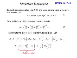
Richardson extrapolation Determining the order of accuracy Assumption:
Richardson extrapolation Three numerical solutions needed Pointwise approach interpolation to a common grid needed
Interpolation Interpolation polynomial: Fifth degree in x and y 36 points • Lagrange interpolation in interior • 6x6 squares • Matrix interpolation near wall • Row Scaling • Shifting interpolation procedure • Using wall condition 6th order interpolation method, tested by analytical testcase
Results Solution at t = 4.2 Order of accuracy at t = 4.2
Results (cont)Impact of boundary condition and filter • Boundary condition • Filter for removing high frequency noise
Results (cont) Order of accuracy t = 8.4 t = 4.2
Results (cont)Impact of outflow condition • Outflow boundary condition • Replace by solid wall
Results (cont)Impact of cut-cell method Order of accuracy t = 8.4 t = 12.6 Solid wall
Results (cont)Impact of cut-cell method fn fe fw • Interpolation method used for and • Tested by analytical testcase • Results obtained with three norms • Order of accuracy about 0!! fsw fe fint fsw
Conclusions • Interpolation to common grid • 6th order to preserve accuracy of numerical solution • Impact of discontinuities and filter • Negative impact on order of accuracy • Impact of outflow boundary conditions • Can handle waves from only one direction • Impact of cut-cell method • Lower order of accuracy due to interpolation • Richardson extrapolation • Only for “smooth” problems