Experiments with Range Computations using Extrapolation
Experiments with Range Computations using Extrapolation. P. S. V. Nataraj And Shanta Sondur Systems & Control Engineering, IIT Bombay. Indian Institute of Technology, Bombay 2004. Overview. Introduction NIE and Uniform Subdivision Objective

Experiments with Range Computations using Extrapolation
E N D
Presentation Transcript
Experiments with Range Computations using Extrapolation P. S. V. Nataraj And Shanta Sondur Systems & Control Engineering, IIT Bombay. Indian Institute of Technology, Bombay 2004
Overview • Introduction • NIE and Uniform Subdivision • Objective • Extrapolation Process – Sequence Transformation • The Richardson Extrapolation Process (REP) • Other Extrapolation Algorithms • Error control in Convergence Acceleration Processes • Brezinski’s Theorem • Proposed Algorithm • Illustrative Example – Vehicle Clutch System • Comparison of proposed method with the existing method and with Globsol • Conclusions
Introduction • We present a new method ‘Extrapolated NIE’ to compute the range enclosure of the functions using the NIE with uniform subdivision and Extrapolation Algorithms such as, Richardson Extrapolation Algorithm (REP). • Aim is to ‘Accelerate the Order of Convergence of the NIE’ by extrapolation.
NIE and Uniform Subdivision • Consider the interval vector With components . • Suppose we uniformly subdivide the interval x using the subdivision factor N, as follows,
NIE continued… • Let be the error interval associated with N partitions of the interval vector x expressed as Define as The excess width is defined as
NIE continued… • The excess width also can be expressed as • The range infimum and range supremum can be expressed as
Order of Convergence of NIE with Uniform Subdivision Process • NIE with uniform subdivision process has linear order of convergence. ‘The excess width goes down linearly with the domain width’.
Objective Acceleration of Linear Convergence Process of NIE with Uniform Subdivision.
Extrapolation Process – Sequence Transformation • Extrapolation Algorithms are popularly used for ‘accelerating’ the convergence of a given sequence. • Let (Sn) be a sequence of (real or complex) numbers converging to S. Extrapolation method transforms the sequence (Sn) into another sequence (Tn) which converges to the same limit S, faster than(Sn).
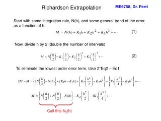
Richardson Extrapolation Algorithm (REP) • Let KN, 2, and {Sn} be the sequence to be accelerated. The REP can be given as
Romberg Table by REP ik =0 k =1 k = 2… 0 A0 (0)2A0(1) – A0(0) A1(0) = (2 –1) 22 A1(1) – A1(0) 1 A0 (1)A2(0) = 2A0(2) – A0(1)(22 –1) A1(1) = (2 –1) 22 A1(2) – A1(1) 2 A0 (2)A2(1) = 2A0(3)– A0(2)(22 –1) A1(2) = (2 –1) 3 A0 (3) O(h) O(h2) O(h3)…
Other Extrapolation Algorithms • Aitkin’s 2 iterated process • Rational Extrapolation • The - algorithm • The E – algorithm • The G - transformation • Levin’s transform • Overholt’s process
Error control in Convergence Acceleration Processes • From user’s point of view it is not sufficient to know that, for a given sequence (Sn), the extrapolated sequence (Tn) will converge faster. • One should have an estimate of the error (Tn – S) or, still better, to know a sequence of intervals containing the unknown limit S of the sequence (Sn). • Brezinski’s method can be used for estimating the error on the transformed sequences (Tn) obtained through Extrapolation process.
Brezinski’s Interval • Let (Tn) and (Vn) be the transformed sequences of (Sn) converging to the same limit S, and let Vn(b) and Jn(b) be defined as
Brezinski’s Theorem If the sequence (Tn) converges to S faster than the original sequence (Sn) with limit S and if the sequence (Vn) converges to S faster than the (Tn),then for all b 0, N:n N, the true valueS will be contained in an interval Jn(b). Moreover, the sequence Vn(b) will converge faster than the (Sn).
Proposed Algorithm • Generate the two separate sequences of Lower and Upper bounds on the range infium and range supremum, respectively. • Apply REP and generate Romberg Tables for range infimum and supremum. • Construct Brezinski’s Tables of intervals approximating the range infimum (BTII) and supremum (BTIS). • Construct the final table of intervals approximating the range from BTII and BTIS.
Procedure to construct the sequences Do j = 1, 2,…,K • Subdivide the box x uniformly into Nj=2j subboxes. Let, • Compute the range enclosure • Set End do
Romberg Table for Infimum k =0 k =1 k = 2….. A0 (0) = inf (F2(X))A0(1) – A0(0) A1(0) = A0(1) + (2k+1 –1) A1(1) – A1(0) A0 (1) = inf (F4(X))A2(0) = A1(1) + A0(2) – A0(1)(2k+1 –1) A1(1) = A0(2) + (2k+1 –1) A1(2) – A1(1) A0 (2) = inf (F8(X))A2(1) = A1(2) + A0(3) – A0(2)(2k+1 –1) A1(2) = A0(3) + (2k+1 –1) A1(3) – A1(2) A0 (3) = inf (F16(X))A2(2) = A1(3) + A0(4) – A0(3)(2k+1 –1) A1(3) = A0(4) + (2k+1 –1) A0 (4) = inf (F32(X))
Romberg Table for Supremum k =0 k =1 k = 2….. A0 (0) = sup (F2(X))A0(1) – A0(0) A1(0) = A0(1) + (2k+1 –1) A1(1) – A1(0) A0 (1) = sup (F4(X))A2(0) = A1(1) + A0(2) – A0(1)(2k+1 –1) A1(1) = A0(2) + (2k+1 –1) A1(2) – A1(1) A0 (2) = sup (F8(X))A2(1) = A1(2) + A0(3) – A0(2)(2k+1 –1) A1(2) = A0(3) + (2k+1 –1) A1(3) – A1(2) A0 (3) = sup (F16(X))A2(2) = A1(3) + A0(4) – A0(3)(2k+1 –1) A1(3) = A0(4) + (2k+1 –1) A0 (4) = sup (F32(X))
Procedure to construct the Brezenski’s Interval • Let Sn = Ak(i), Tn = Ak+1(i), and Vn = Ak+2(i), k=1,2,…,K and i = k,…,K, and b = 1. • Construct Brezenski’s Interval Jn(b) for the entries in the Romberg Table for Infimum and Supremum. • Call the resulting table as Brezenski’s Table of Intervals for Infimum (BTII) and Brezenski’s Table of Intervals for Supremum (BTIS). • Construct the range enclosure by F(X) = [inf(BTII), sup(BTIS)].
engine Illustrative ExampleVehicle Clutch System jc je Cs jv load Te gr fuel Ks Cpos Vehicle Driveline Model
Parameters of Vehicle Parameter Symbols Range of Values Clutch inertia jc 0.09 kg m2 Engine inertia je 3.07 kg m2 Vehicle inertia jv [1400, 11000] kg m2 Axle shaft spring rate ks [58000, 115000] N m/rad Axle and tyre damping Cc 377 N m/rad/s Engine viscous friction Ce 18.5 N m/rad/s Overall gear ratio gr 27.0 Clutch torque Kc [100, 800]N m/mm Cpos
Transfer function • Three uncertain physical parameters are: • vehicle inertia jv, • axel shaft spring rate, ks, and • the ratio between change in clutch torque and change in clutch position, Kc. The transfer function between the clutch position Cpos and the transmission input speed Si is given as:
Magnitude Function With parameter uncertainties as follows: for frequency =50.
Range computed using NIE and Uniform subdivision True_range = [ 64.17591070389160, 92.11586932433393] N Range computed using NIE and Uniform subdivision 64 [ 63.30270186117932, 92.43277538797648] 128 [ 63.72755957264531, 92.17531914664293] 256 [ 63.94859696170153, 92.14554381891074] 512 [ 64.06144077281130, 92.13069401039323] 1024 [ 64.11846865754421, 92.12327853239701] 2048 [ 64.14713741612914, 92.11957314529018] 4096 [ 64.16151093091627, 92.11772103912668] 8192 [ 64.16870752718803, 92.11679513281965]
Romberg Table for Infimum K=0 K=1 K=2 K=3 • 63.30270186117932 • 63.72755957264531 64.15241728411131 • 63.94859696170154 64.16963435075778 64.17537337297326 • 64.06144077281131 64.17428458392108 64.17583466164219 64.17590056002345 • 64.11846865754423 64.17549654227715 64.17590052839584 64.17590993793208 • 64.14713741612916 64.17580617471408 64.17590938552640 64.17591065083076 • 64.16151093091628 64.17588444570340 64.17591053603319 64.17591070039130 • 64.16870752718805 64.17590412345982 64.17591068271196 64.17591070366606 K=4 K=5 K=6 K=7 • 64.17591056312600 • 64.17591069835733 64.17591070271963 • 64.17591070369534 64.17591070386753 64.17591070388575 • 64.17591070388438 64.17591070389048 64.17591070389084 64.17591070389088
BTII for Infimum i K=1 K=2 K=3 • [ 63.9485, 64.3907] • [ 64.0614, 64.2872] [ 64.1742, 64.1774] • [ 64.1184, 64.2326] [ 64.1754, 64.1764] [ 64.1759, 64.1760] • [ 64.1471, 64.2045] [ 64.1758, 64.1761] [ 64.1759, 64.1760] • [ 64.1615, 64.1903] [ 64.1758, 64.1760] [ 64.1759, 64.1760] • [ 64.1687, 64.1832] [ 64.1759, 64.1760] [ 64.1759, 64.1760] K=4 K=5 K=6 • [ 64.1759, 64.1760] • [ 64.1759, 64.1760] [ 64.1759, 64.1760] • [ 64.1759, 64.1760] [ 64.1759, 64.1760] [ 64.1759, 64.1760]
Overestimation and Ratio for BTII Overestimation i k=1 k=2 k=3 k=4 k=5 max (true) max (true) max (true) max (true) max (true) • 4.4e-1(2.3e-1) • 2.3e-1(1.1e-1) 3.1e-3(1.6e-3) • 1.1e-1(5.7e-2) 8.1e-4(4.1e-4) 1.9e-5(1.0e-5) • 5.7e-1(2.9e-2) 2.1e-4(1.0e-4) 2.5e-6(1.3e-6) 9.5e-08(5.3e-08) • 2.9e-1(1.4e-2) 5.2e-5(2.6e-5) 3.3e-7(1.7e-7) 6.6e-09(3.5e-09) 3.4e-10(1.9e-10) • 1.4e-2(7.2e-3) 1.3e-5(6.6e-6) 4.2e-8(2.1e-8) 4.4e-10(2.3e-10) 1.2e-11(7.3e-12) Overestimation Ratio i k=1 k=2 k=3 k=4 k=5 • 1.9858 • 1.9928 3.9263 • 1.9964 3.9622 7.7183 • 1.9982 3.9808 7.8540 15.158 • 1.9991 3.9903 7.9254 15.515 26.787 O(21=2) O(22=4) O(23=8) O(24=16) O(25=32)
Romberg Table for Supremum K=0 K=1 K=2 K=3 • 92.43277538797648 • 92.17531914664292 91.91786290530936 • 92.14554381891072 92.11576849117853 92.18173701980159 • 92.13069401039321 92.11584420187570 92.11586943877477 92.10645978434236 • 92.12327853239701 92.11586305440081 92.11586933857585 92.11586932426171 • 92.11957314529018 92.11586775818334 92.11586932611085 92.11586932433013 • 92.11772103912668 92.11586893296318 92.11586932455647 92.11586932433441 • 92.11679513281965 92.11586922651262 92.11586932436244 92.11586932433471 K=4 K=5 K=6 K=7 • 92.11649662692301 • 92.11586932433470 92.11584908876733 • 92.11586932433470 92.11586932433470 92.11586964553419 • 92.11586932433474 92.11586932433474 92.11586932433474 92.11586932180560
BTIS for Supremum K=1 K=2 K=3 • [ 92.0859, 92.1456] • [ 92.1009, 92.1307] [ 92.1158, 92.1159] • [ 92.1084, 92.1233] [ 92.1158, 92.1159] [ 92.1158, 92.1159] • [ 92.1121, 92.1196] [ 92.1158, 92.1159] [ 92.1158, 92.1159] • [ 92.1140, 92.1178] [ 92.1158, 92.1159] [ 92.1158, 92.1159] • [ 92.1149, 92.1168] [ 92.1158, 92.1159] [ 92.1158, 92.1159] K=4 • [ 92.1158, 92.1159] • [ 92.1158, 92.1159] • [ 92.1158, 92.1159]
Overestimation and Ratio for BTIS Overestimation i k=1 k=2 k=3 k=4 max (true) max (true) max (true) max (true) • 6.0e-02(3.0e-02) • 3.0e-02(1.5e-02) 5.0e-05(2.5e-05) • 1.5e-02(7.4e-03) 1.3e-05(6.3e-06) 2.9e-08(1.4e-08) • 7.4e-03(3.7e-03) 3.1e-06(1.6e-06) 3.6e-09(1.8e-09) (9.3e-12)(5.4e-12) • 3.7e-03(1.9e-03) 7.8e-07(3.9e-07) 4.4e-10(2.2e-10) (*)(1.1e-12) • 1.9e-03(9.3e-04) 2.0e-07(9.8e-08) 5.6e-11(2.9e-11) (*)(8.8e-13) Overestimation Ratio i k=1 k=2 k=3 k=4 • 2.0017 • 2.0008 4.0250 • 2.0004 4.0125 8.0148 • 2.0002 4.0062 7.9838 - • 2.0001 4.0031 7.7998 - O(21=2) O(22=4) O(23=8) (*) – denotes the zero within machine precision.
Range Enclosures: [inf(BTII), sup(BTIS)] i k=0 k=1 • [ 63.30270186117932, 92.43277538797648] • [ 63.72755957264531, 92.17531914664293] • [ 63.94859696170153, 92.14554381891074] [ 63.94859696170151, 92.14554381891074] • [ 64.06144077281130, 92.13069401039323] [ 64.06144077281130, 92.13069401039323] • [ 64.11846865754421, 92.12327853239701] [ 64.11846865754421, 92.12327853239701] • [ 64.14713741612914, 92.11957314529018] [ 64.14713741612914, 92.11957314529018] • [ 64.16151093091627, 92.11772103912668] [ 64.16151093091627, 92.11772103912668] • [ 64.16870752718803, 92.11679513281965] [ 64.16870752718803, 92.11679513281965] i k=2 k=3 • [ 64.17428458392106, 92.11589467567383] • [ 64.17549654227713, 92.11587562275091] [ 64.17590052839580, 92.11586933857588] • [ 64.17580617471405, 92.11587089403837] [ 64.17590938552633, 92.11586932611090] • [ 64.17588444570338, 92.11586971614976] [ 64.17591053603312, 92.11586932455650] • [ 64.17590412345980, 92.11586942221226] [ 64.17591068271190, 92.11586932436248] i k=4 • [ 64.17591065083067, 92.11586932433933] • [ 64.17591070039119, 92.11586932433507] • [ 64.17591070366599, 92.11586932433481]
True Range Overestimation and Ratio Overestimation i k=1 k=2 k=3 k=4 k=5 • 1.2 • 5.1e-01 • 2.6e-01 2.6e-01 • 1.3e-01 1.3e-01 1.7e-03 • 6.5e-02 6.5e-02 4.2e-04 1.0e-05 • 3.2e-02 3.2e-02 1.1e-04 1.3e-06 5.3e-08 • 1.6e-02 1.6e-02 2.7e-05 1.7e-07 3.5e-09 • 8.1e-03 8.1e-03 6.7e-06 2.1e-08 2.3e-10 Overestimation Ratio i k=1 k=2 k=3 k=4 k=5 • 2.3437 • 1.9760 • 1.9876 1.9876 • 1.9937 1.9937 3.9278 • 1.9968 1.9968 3.9629 7.7187 • 1.9984 1.9984 3.9812 7.8542 15.155 • 1.9992 1.9992 3.9905 7.9253 15.460 O(21=2) O(22=4 ) O(23=8) O(24=16) O(25=32 )
Comparison of Existing method with the proposed method • Number of subdivisions required and number of boxes generated to compute the Bode magnitude envelope with accuracy = 10-10. Existing Method Proposed method Subdivision factors 240 213 Number of Boxes 4974 4872 in the final list (with cutoff test) Time (sec.) 24.6 4.9
Comparison of the proposed method with Globsol • Time (sec.) required to compute the Bode magnitude envelope with accuracy = 10-10. Proposed method Globsol 4.9 sec. 19.18 sec.
Conclusions • We could Accelerate the order of Convergence of NIE by Extrapolation. • The width of the Brezinski’s intervals is a good measure of having attained the specified accuracy • High accuracy can be achieved with comparatively less computational effort! • In the vehicle clutch example: • Number of subdivisions required to compute the Range enclosure with the proposed method is significantly reduced. • The proposed method is faster compared with Globsol.

