MITM 613 Intelligent System
420 likes | 577 Views
MITM 613 Intelligent System. Chapter 8a: Support Vector Machine. Chapter Eight(a) : SVM. Introduction Theory Implementation Tools Comparison LIBSVM practical. Introduction (1 of 9). Introduction (1). SVM is mainly used in the problem of classification and regression .

MITM 613 Intelligent System
E N D
Presentation Transcript
MITM 613Intelligent System Chapter 8a: Support Vector Machine
Chapter Eight(a) : SVM • Introduction • Theory • Implementation • Tools Comparison • LIBSVM practical Abdul Rahim Ahmad
Introduction (1 of 9) Introduction (1) • SVM is mainly used in the problem of classification and regression. • In classification, • We want to estimate a decision function, f using a set of training data with labels such that f will correctly classify unseen test examples. • Definition of SVM: • “The Support Vector Machine is a learning machine for pattern recognition and regression problems which constructs its solution (decision function f) in terms of a subset of the training data, the Support Vectors.”
Introduction (1 of 9) Introduction (2) • Why the name machine? • Implemented in Software – a software machine • It receive input and produce output – classification. • What are support vectors? • A (small) subset of the set of input vectors that are needed for the final machine implementation. ie: they support the final machine functionality. • What relation with Neural Network (NN)? • It perform similar function as NN – pattern recognition, function estimation, interpolation, regression etc. • Only BETTER.
Introduction (3) Introduction (3 of 9) • History • SVM came from the idea of "Generalized Portrait" Algorithm in 1963 for constructing separating hyperplanes with optimal margin. • Introduced as Large Margin classifier in the COLT 1992 conference by Boser, Guyon,Vapnik in the paper:“A Training Algorithm for Optimal Margin Classifiers. “ • What is Optimal margin classifier? • Classification algorithm that maximize the margin between nearest points on separate classes in the classification.
Introduction (4) Introduction (4 of 9) • Why the need to achieve optimal margin? • Optimal margin leads to better generalization • Implying minimization of overall risk • Two kinds of Risk Minimization : • Structural Risk Minimization (SRM) • As in SVM • Empirical Risk Minimization (ERM) • As in Neural Network
Introduction (5 of 9) Introduction (5) • What is Risk minimization ? • choosing appropriate value for parameters, eg: α that minimize: • where • α defines the parameterisation • Q is the loss function • z belongs to the union of input and output spaces • P describes the distribution of z • P can only be estimated – normally avoided (to simplify) by using empirical risk: • Minimizing this is called empirical risk minimisation (as in NN).
Introduction (6 of 9) Introduction (6) • Vapnik (Vapnik, 1995) proved that the bound on expected risk is: • Where h, is the VC dimension – measure of the capacity of the learning machine. f(h) provides the confidence in the risk. • SRM identify optimal point on the curve for bound on the expected risk (ie:trade-off between expected risk and complexity of the approximating function)
Introduction (7 of 9) Introduction (7) • Risk minimization - two distinct ways • Fix confidence in the risk, optimize empirical risk - Neural network. • Fix empirical risk, optimize confidence interval - SVM. • In NN: Fix network structure. learning -> minimize empirical risk.(using gradient descent) • In SVM: Fix empirical risk.(to min, or 0 for separable data set), learning -> optimizes for a minimum confidence interval (maximizing the margin of the separating hyper plane).
Introduction (8 of 9) Introduction (8) • To implemet SRM -> Find Largest margin by either of the following methods FindOptimal plane that maximize margin Find Optimal plane that bisects closest points in convex hulls More often used
NN 1 NN 2 D B C A A, B, C, D are the Support Vectors Optimal decision function Have large margin between nearest points of the 2 classes Introduction (9 of 9) Introduction (9) • Most popular classifiers are trained using Neural network (NN). • NN decision function might not be • the same for every training and for different initial parameter values • Optimal since training stops once convergence is achieved • For better generalization, we need optimal decision function – the one and only.
Theory (1/15) Theory (1) • 3 cases of SVM : • Linearly separable case. • Non-linearly separable case. • Non-separable or imperfect separation case (allowing for noise).
H1: y = w.x + b = +1 H: y = w.x + b = 0 H2: y = w.x + b = -1 Theory (2/15) Theory (2) • Linearly separable case. • Specifically we want to find a plane H: y = w.x + b = 0 and two planes parallel to it, say H1 and H2 such that they are equidistant from H and H1: y = w.x + b = +1 and H2: y = w.x + b = -1 . • Also there should be no data points between H1 and H2 and the distance M between H1 and H2 is maximized.
H1: y = w.x + b = +1 H: y = w.x + b = 0 H2: y = w.x + b = -1 Theory (3/15) Theory (3) • The distance of a point on H1 to H is : • |w.x + b|/||w|| = 1/||w||, • Therefore the distance between H1 and H2 is 2/||w||
H1: y = w.x + b = +1 H: y = w.x + b = 0 H2: y = w.x + b = -1 Theory (4/15) Theory (4) • In order to maximize the distance we minimize ||w||. Furthermore we do not want any data points between the two. Thus we have : • H1: y = w.x + b +1 for positive examples yi = +1 • H2: y = w.x + b -1 for negative examples yi = -1 • The two equations can be combined: yi (w.x + b) 1 • Formulation for Optimal Hyper plane is : Minimize ||w||subject to yi (w.x + b) 1
Theory (5/15) Theory (5) • This is a convex, quadratic programming problem (in w, b) in a convex set, which can be solved by introducing N non-negative Lagrange multipliers 1, 2,…, N 0 associated with the constraints. (Theory of Lagrange Multipliers) • Thus we have the following Lagrangian to solve for i’s : • We have to minimize this function over w and b and maximize it over i’s. • We can solve the Wolfe dual of the Langrangian, instead : • Maximize L(w, b, ) w.r.t , subject to the constraints that the gradient of L(w, b, ) w.r.t to the primal variables w and b vanish ie: L/ w = 0 and L/ b = 0 and that 0. • We thus have and
Theory (6/15) Theory (6) • Putting and in L(w, b, ), we get the wolfe dual: in which input data only appear in a dot product. • We solve for i’s which will maximize Ld subject to I ≥ 0 i=1,…,l and • The hyperplane decision function is thus : or • Since I ≥ 0 for all points on the margin and I = 0 for others, only those I play a role in the decision function. They are called support vectors • The number of support vectors are usually small, thus we say that the solution to SVM is sparse.
Theory (7/15) Theory (7) • Non linear (separable) case • In this case, we can transform the data points into another high dimensional space such that the data points will be linearly separable in the new space. We construct Optimal Separating Hyper plane in that space. • Let the transformation be (.). In the high dimensional space, we solve: • Example of mappingfrom 2D to3D
Theory (8/15) Theory (8) • Non linear (separable) case • In place of the dot product, if we can find a kernel function which perform this dot product implicitly, we can replace it with that kernel (ie: perform kernel evaluation instead of explicitly map the training data) • The hyper plane decision function is thus now :
Theory (9/15) Theory (9) SVM for Non-linear Separable Case An SVM corresponds to a non-linear decision surface in input surface R2 Data points in input space Mapping from R2via into R3 Hyperplane in feature space R3
Theory (10/15) Theory (10) • Non linear (separable) case • To determine if a dot product in high dimensional space is equivalent to a kernel function in input space, i.e: (xi).(xj) = K(xi.xj) • Use Mercer’s condition • Need not have to be explicit about the transformation (.) as long as we know that K(xi.xj) is equivalent to the dot product of some other high dimensional space. • Kernel functions that can be used this way: • Linear kernel • Polynomial kernels • Radial basis function (Gaussian kernel) • Hyperbolic tangent kernel
Theory (11/15) Theory (11) Imperfect Separation Case • No strict enforcement that there be no data points between hyperplanes H1 and H2 • But penalize the data points that are in the wrong side. • Penalty C is finite and have to be chosen by the user. Large C means higher penalty. • We introduce non-negative slack variable 0 so that : • W.xi + b + 1 - i for yi = +1 • W.xi + b - 1 + i for yi = -1 0 i.
Theory (12/15) Theory (12) • We add to the objective function a penalising term • Where m is usually set to 1, which gives ussubject to
Theory (13/15) Theory (13) Imperfect Separation Case • Introducing Lagrange multipliers , , the lagrangian is: • Similarly, solving for the Wolfe dual, neither I nor their Lagrange multipliers, appear in the dual problem. Minimize Subject to 0 i C and • The only difference from the perfectly separating case is that I now is bounded by C. The solution is again given by
Most commonly used Theory (14/15) Theory (14) • Different SVM Objective functions leads to different SVM variations • Using l1 norm • Using l2norm • Using l1 norm for w - linear programming (LP) SVM • v parameter for controlling the number of support vectors
Theory (15/15) Theory (15) • SVM architecture (for Neural Network users) • The kernel function k is chosen a priori (determine the type of classifier). • Training – solve a quadratic programming problem to find • no of hidden units (no. of support vectors), • weights (w), • threshold (b) • The first layer weights xi are a subset of the training set (the support vectors). • The second layer weights I = yi I are computed from the Lagrange Multipliers.
Application (1/1) Application (1) • SVM Applications • applied to a number of applications such as • Image classification. • Time series prediction • Face recognition • Biological data processing for medical diagnosis • Digit recognition (MLP-SVM) • Text Categorisation • Speech recognition • Using hybrid SVM/HMM
Implementation (1/6) Implementation (1) • SVM Implementation • High-performance classifiers • use of kernels. • Different kernel functions lead to • very similar classification accuracies • produced similar SV sets. (that is the SV set seems to characterize the given task up to a certain degree independent of the type of kernel)
Implementation (2/6) Implementation (2) • SVM Implementation • Main issues are classification accuracy and speed • To improve on the speed, a number of improvements to original SVM are developed: • (1) Chunking - Osuna • (2) Sequential Minimization Optimization(SMO) - Platt (1) Nearest Point Algorithm – Keerthi
Implementation (3/6) Implementation (3) SVM Software Implementation • In high level languages C, C++, FORTRAN • SVM light - Thorsten Joachims'. • mySVM -Ruping • SMO in C++ - XiaPing Yi • LIBSVM – Chih Jen Lin • Matlab, toolbox • OSU SVM Toolbox - Junshui Ma and Stanley Ahalt. • MATLAB Support Vector Machine Toolbox - Gavin Cawley • Matlab routines for support vector machine classification - Anton Schwaighofer • MATLAB Support Vector Machine Toolbox - Steve Gunn • LearnSC - Vojislav Kecman • LIBSVM Interface – students of C.J.Lin
Implementation (4/6) Implementation (4) • Steps in SVM training • Select the parameter C (representing the tradeoff between minimizing the training error and margin maximization), kernel function and any kernel parameters. • Solve the dual QP or alternative problem formulation using appropriate QP or LP algorithm to obtain the support vectors. • Calculate threshold b using the support vectors.
Implementation (5/6) Implementation (5) • Model Selection: • Minimizing an estimate of generalization error or some related performance measures • K-fold cross-validation and leave-one-out (LOO) estimates • Other recent model selection strategies are based on some bound determined by a quantity (through theoretical analysis) which is not obtained using retraining with data points left out (as in cross-validation or LOO) • SV count /Jaakkola Haussler bound /Opper – Winther Bound/ Radius – margin Bound /Span Bound/ • 10-fold cross-validation is popularly used and used in my work.
Implementation (6/6) Implementation (6) • Different methods for QP Optimization: • (a) techniques in which kernel components are evaluated and discarded during learning Kernel Adatron • (b) decomposition method in which an evolving subset of data is used and Sequential Minimal Optimization (SMO) SVMlight/LIBSVM • (c) new optimization approaches that specifically exploit the structure of the SVM problem. Nearest point algorithm (NPA)
Implementation (III) SVMTORCH
Implementation (III) SVMLight
Implementation (III) LIBSVM
LIBSVM History • 1.0 : June 2000 First Release. • 2.0 : Aug 2000 Major updates – add nu-svm, one-class svm, and svr • 2.1 : Dec 2000 Java version added, regression demonstrated in svm-toy • 2.2 : Jan 2001 Multi-class classification, nu-SVR • 2.3 : Mar 2001 Cross validation, fix some minor bugs • 2.31: April 2001 Fix one bug on one-class SVM, use float for Cache • 2.33: Dec 2001 Python interface added • 2.36: Aug 2002 grid.py added: contour plot of CV accuracy • 2.4 : April 2003 improvements of scaling • 2.5 : Nov 2003 some minor updates • 2.6 : April 2004 Probability estimates for classification/regression • 2.7 : Nov 2004 Stratified cross validation • 2.8 : April 2005 New working set selection via second order information
LIBSVM Current Version • 2.81: Nov 2005 • 2.82: Apr 2006 • 2.83: Nov 2006 • 2.84: April 2007 • 2.85: Nov 2007 • 2.86: April 2008 • 2.87: October 2008 • 2.88: October 2008 • 2.89: April 2009 • 2.9: November 2009 • 2.91: April 2010 • 3.0 : September 13, 2010 • 3.12: April Fools' day, 2012 http://www.csie.ntu.edu.tw/~cjlin/libsvm/
LIBSVM for Windows • Java • C/C++ • LIBSVM in MATLAB • LIBSVM in R package • LIBSVM in WEKA