Download
1 / 61
610 likes | 645 Views
Learn about power grid operation, transmission system impact, and basic power flow concepts through simulations in PowerWorld Simulator. Explore generation, load, transmission components, and power balance constraints.

E N D
How the Power Grid Behaves Tom Overbye Department of Electrical and Computer Engineering University of Illinois at Urbana-Champaign
Presentation Overview • Goal is to demonstrate operation of large scale power grid. • Emphasis on the impact of the transmission syste. • Introduce basic power flow concepts through small system examples. • Finish with simulation of Eastern U.S. System.
PowerWorld Simulator • PowerWorld Simulator is an interactive, Windows based simulation program, originally designed at University of Illinois for teaching basics of power system operations to non-power engineers. • PowerWorld Simulator can now study systems of just about any size.
Eastern Interconnect Operating Areas Ovals represent operating areas Arrows indicate power flow in MW between areas
Power System Basics • All power systems have three major components: Generation, Load and Transmission. • Generation: Creates electric power. • Load: Consumes electric power. • Transmission: Transmits electric power from generation to load.
One-line Diagram • Most power systems are balanced three phase systems. • A balanced three phase system can be modeled as a single (or one) line. • One-lines show the major power system components, such as generators, loads, transmission lines. • Components join together at a bus.
Eastern North American High Voltage Transmission Grid Figure shows transmission lines at 345 kV or above in Eastern U.S.
Zoomed View of Midwest Arrows indicate MW flow on the lines; piecharts show percentage loading of lines
Example Three Bus System Pie charts show percentage loading of lines Generator Load Bus Circuit Breaker
Generation • Large plants predominate, with sizes up to about 1500 MW. • Coal is most common source, followed by hydro, nuclear and gas. • Gas is now most economical. • Generated at about 20 kV.
Loads • Can range in size from less than a single watt to 10’s of MW. • Loads are usually aggregated. • The aggregate load changes with time, with strong daily, weekly and seasonal cycles.
Transmission • Goal is to move electric power from generation to load with as low of losses and cost as possible. • P = V I or P/V = I • Losses are I2 R • Less losses at higher voltages, but more costly to construct and insulate.
Transmission and Distribution • Typical high voltage transmission voltages are 500, 345, 230, 161, 138 and 69 kV. • Transmission tends to be a grid system, so each bus is supplied from two or more directions. • Lower voltage lines are used for distribution, with a typical voltage of 12.4 kV. • Distribution systems tend to be radial. • Transformers are used to change the voltage.
Other One-line Objects • Circuit Breakers - Used to open/close devices; red is closed, green is open. • Pie Charts - Show percentage loading of transmission lines. • Up/down arrows - Used to control devices. • Values - Show current values for different quantities.
Power Balance Constraints • Power flow refers to how the power is moving through the system. • At all times the total power flowing into any bus MUST be zero! • This is know as Kirchhoff’s law. And it can not be repealed or modified. • Power is lost in the transmission system.
Basic Power Control • Opening a circuit breaker causes the power flow to instantaneously(nearly) change. • No other way to directly control power flow in a transmission line. • By changing generation we can indirectly change this flow.
Flow Redistribution Following Opening Line Circuit Breaker No flow on open line Power Balance must be satisfied at each bus
Indirect Control of Line Flow Generator change indirectly changes line flow Generator MW output changed
Transmission Line Limits • Power flow in transmission line is limited by a number of considerations. • Losses (I2 R) can heat up the line, causing it to sag. This gives line an upper thermal limit. • Thermal limits depend upon ambient conditions. Many utilities use winter/summer limits.
Overloaded Transmission Line Thermal limit of 150 MVA
Interconnected Operation • Power systems are interconnected across large distances. For example most of North American east of the Rockies is one system, with most of Texas and Quebec being major exceptions • Individual utilities only own and operate a small portion of the system, which is referred to an operating area (or an area).
Operating Areas • Areas constitute a structure imposed on grid. • Transmission lines that join two areas are known as tie-lines. • The net power out of an area is the sum of the flow on its tie-lines. • The flow out of an area is equal to total gen - total load - total losses = tie-flow
Three Bus System Split into Two Areas Initially area flow is not controlled Net tie flow is NOT zero
Area Control Error (ACE) • The area control error mostly the difference between the actual flow out of area, and scheduled flow. • ACE also includes a frequency component. • Ideally the ACE should always be zero. • Because the load is constantly changing, each utility must constantly change its generation to “chase” the ACE.
20.0 10.0 0.0 Area Control Error (MW) -10.0 -20.0 06:30 AM 06:15 AM Time Home Area ACE ACE changes with time
Inadvertent Interchange • ACE can never be held exactly at zero. • Integrating the ACE gives the inadvertent interchange, expressed in MWh. • Utilities keep track of this value. If it gets sufficiently negative they will “pay back” the accumulated energy. • In extreme cases inadvertent energy is purchased at a negotiated price.
Automatic Generation Control • Most utilities use automatic generation control (AGC) to automatically change their generation to keep their ACE close to zero. • Usually the utility control center calculates ACE based upon tie-line flows; then the AGC module sends control signals out to the generators every couple seconds.
Three Bus Case on AGC With AGC on, net tie flow is zero, but individual line flows are not zero
Generator Costs • There are many fixed and variable costs associated with power system operation. • Generation is major variable cost. • For some types of units (such as hydro and nuclear) it is difficult to quantify. • For thermal units it is much easier. There are four major curves, each expressing a quantity as a function of the MW output of the unit.
Generator Cost Curves • Input-output (IO) curve: Shows relationship between MW output and energy input in Mbtu/hr. • Fuel-cost curve: Input-output curve scaled by a fuel cost expressed in $ / Mbtu. • Heat-rate curve: shows relationship between MW output and energy input (Mbtu / MWhr). • Incremental (marginal) cost curve shows the cost to produce the next MWhr.
10000 7500 5000 Fuel-cost ($/hr) 2500 0 0 150 300 450 600 Generator Power (MW) Example Generator Fuel-Cost Curve Y-axis tells cost to produce specified power (MW) in $/hr Current generator operating point
20.0 15.0 Incremental cost ($/MWH) 10.0 5.0 0.0 0 150 300 450 600 Generator Power (MW) Example Generator Marginal Cost Curve Y-axis tells marginal cost to produce one more MWhr in $/MWhr Current generator operating point
Economic Dispatch • Economic dispatch (ED) determines the least cost dispatch of generation for an area. • For a lossless system, the ED occurs when all the generators have equal marginal costs.IC1(PG,1) = IC2(PG,2) = … = ICm(PG,m)
Power Transactions • Power transactions are contracts between areas to do power transactions. • Contracts can be for any amount of time at any price for any amount of power. • Scheduled power transactions are implemented by modifying the area ACE:ACE = Pactual,tie-flow - Psched
Implementation of 100 MW Transaction Overloaded line Net tie flow is now 100 MW from left to right Scheduled Transaction
Security Constrained ED • Transmission constraints often limit system economics. • Such limits required a constrained dispatch in order to maintain system security. • In three bus case the generation at bus 3 must be constrained to avoid overloading the line from bus 2 to bus 3.
Security Constrained Dispatch Gens 2 &3 changed to remove overload Net tie flow is still 100 MW from left to right
Multi-Area Operation • The electrons are not concerned with area boundaries. Actual power flows through the entire network according to impedance of the transmission lines. • If Areas have direct interconnections, then they can directly transact up their tie-line capacity. • Flow through other areas is known as “parallel path” or “loop flows.”
Seven Bus, Thee Area Case One-line Area “Top” has 5 buses ACE for each area is zero Area “Left” has one bus Area “Right” has one bus
Seven Bus Case: Area View Actual flow between areas Scheduled flow between areas
Seven Bus Case with 100 MW Transfer Losses went up from 7.09 MW 100 MW Scheduled Transfer from Left to Right
Seven Bus Case One-line Transfer also overloads line in Top
Transmission Service • FERC Order No. 888 requires utilities provide non-discriminatory open transmission access through tariffs of general applicability. • FERC Order No. 889 requires transmission providers set up OASIS (Open Access Same-Time Information System) to show available transmission.
Transmission Service • If areas (or pools) are not directly interconnected, they must first obtain a contiguous “contract path.” • This is NOT a physical requirement. • Utilities on the contract path are compensated for wheeling the power.
Eastern Interconnect Example Arrows indicate the basecase flow between areas
Power Transfer Distribution Factors (PTDFs) • PTDFs are used to show how a particular transaction will affect the system. • Power transfers through the system according to the impedances of the lines, without respect to ownership. • All transmission players in network could be impacted, to a greater or lesser extent.
PTDFs for Transfer from Wisconsin Electric to TVA Piecharts indicate percentage of transfer that will flow between specified areas
PTDF for Transfer from WE to TVA 100% of transfer leaves Wisconsin Electric (WE)
PTDFs for Transfer from WE to TVA About 100% of transfer arrives at TVA But flow does NOT follow contract path