Download
1 / 20
200 likes | 346 Views
CSC407: Software Architecture Fall 2006 Performance (III). Amit Chandel & Greg Wilson amit@cs.toronto.edu gvwilson@cs.utoronto.ca. Model Revisited. Service Rate μ. FCFS. Arrival Rate λ. Queue. Server. μ. μ. μ. μ. μ. μ. 1. 2. λ. 0. 1. 3. 4. 5. 6. λ. λ. λ. λ. λ.

E N D
CSC407: Software ArchitectureFall 2006Performance (III) Amit Chandel & Greg Wilson amit@cs.toronto.edu gvwilson@cs.utoronto.ca
Model Revisited Service Rate μ FCFS Arrival Rate λ Queue Server μ μ μ μ μ μ 1 2 λ 0 1 3 4 5 6 λ λ λ λ λ
Generalized Birth-Death Models • A restricted class of Markov models 1 2 3 0 0 1 2 3 … 1 2 3 0
M/M/1 System – Steady State μ μ μ μ μ μ 1 2 λ 0 1 3 4 5 6 λ λ λ λ λ
…M/M/1 System – Steady State Let us solve:
Utilization: U = 1 – π0 = Conventional to use for utilization instead of U Number of customers in whole system: …M/M/1 System – Performance Measures
Mean Response Time: Little’s Law: E[Ns] = λ E[Ts] …M/M/1 System – Performance Measures
Mean Wait Time in queue (Tw = TQ): Number of jobs waiting in queue Nw: Using Little’s Law: E[Nw] = E[Tw] = 2 / (1 - ) …M/M/1 System – Performance Measures
Example: 1 • File server: 30 requests/sec, 15 msec/request • What is the average response time? • What would it be if the arrival rate doubled? • Assume requests are independent (must verify) • Utilization = E[S] = 0.45 • So average response time is E[S]/(1 - ) = 0.027 sec • At 60 requests/sec, response time is 0.15 sec • Doubling request rate increased response time by 5.6!
Example: 2 • If both the arrival rate and the service rate are doubled, how does the utilization, throughput, mean response time, and average number of jobs in the system change? • Utilization (U)? • Throughput (X)? • Mean Response Time (E[Ts]) ? • Average number of jobs in the system (E[Ns]) ?
Mean Value Analysis • Markov models suffer from state explosion • In practice, easier to calculate loads using an induction technique called Mean Value Analysis • If you response times and throughputs for a population of N customers, it’s easy to calculate the values for N+1 customers • Iterate until either: • All customers are accounted for • Throughputs and response times converge
…Mean Value Analysis Initialize ave. number of customers at device i: ñi(0) = 0 For n = 1, 2, 3, …, calculate: Average residence time for device: Ri(n) = ViSi[1+ ñi(n-1)] = Di[1+ni(n-1)] Overall system response time: R0(n) = ΣViRi(n) Overall system throughput: X0(n) = n / R0(n) Throughput for each device: Xi(n) = ViX0(n) Utilization for each device: Ui(n) = SiXi(n) Average number of customers at each device: ñi(n) = X0(n)Ri(n)
Example fast disk CPU slow disk
…Example • At most 2 users at any time • Because of high demand, there are always 2 users • Each transaction alternates between CPU and disk • Typical transaction requires a total of 10 sec of CPU • Fast disk is twice as fast as the slow one • Transactions spread evenly across disks • Fast disk takes average of 15 seconds to access files • Slow disk takes average of 30 seconds to access files • What happens if we allow 3 concurrent users?
…Example • It’s a little tedious, but that’s what computers are for
Conclusion • Measure, then model, then tune • To tune the micro-level: • Choose the right algorithm • Squeeze it 'til it squeaks • To tune the macro-level: • Eliminate latency, contention, and copying • Micro-tuning will not fix macro problems • But fixing macro problems can make micro problems go away
When Do You Stop? • An optimization problem on its own • Time invested vs. likely performance improvements • Plan A: stop when you satisfy SLAs • Or beat them—always nice to have some slack • Plan B: stop when there are no obvious targets • Flat performance profiles are hard to improve • Plan C: stop when you run out of time • Plan D: stop when performance is "good enough"