Finding Approximately Repeated Data
Learn about the two most common similarity search variants - k-nearest neighbor search and range search. Explore the new variant of similarity join. Discover how to find the closest pairs of data points or the nearest neighbors for a given dataset.

Finding Approximately Repeated Data
E N D
Presentation Transcript
The two most common similarity search variants are: • K nearest neighbor search. Find me the five closest Starbucks to my office. • Range search. Find me all Starbucks within 4 miles of my office. New variant • Similarity Join. Given this set of 12,000 Starbucks, find me the pair that is the closest to each other. Or • For all 12,000 Starbucks, find me their 1-nearest neighbor
Let us review the matrix view of the world Many datasets naturally are, or can be converted into, sparse matrices.
Examples: • The rows are patients, the columns are the drugs they have taken. • The rows are Netflix users, the columns are the movies they purchased. • The rows are animals, the columns are the genes they have. • The rows are documents, the columns are words (or shingles). • Note: • The dimensionally can be very high, there are 1.7 million movies on IMDB • The numerosity can be very high, there are 44 million US Netflix users. • The data is generally very very sparse (sparser than my example below)
Note: These matrices are sets, not lists. You can permute the rows or columns, it makes no difference.
It is possible that some datasets are not Boolean. For example, they cells might contain the users ranking of movies. Surprisingly, we rarely care! The Boolean version of the matrix is good enough for almost everything we want to do. If they are counts, not Boolean, we call them bags.
We can look at the data in two different ways, by row or by column. Note that User 3 and User 5 have very similar tastes in movies (we will define similar later) This could be an exploitable fact. For example , User 3 has not yet seen Movie C6, we could suggest it to her as “you might also like…” .
We can look at the data in two different ways, by row or by column. Note that Movie 1 and Movie 15 are similar, because they are liked by they same people (we will define similar later). These is also exploitable in many ways.
Getting data in the matrix format Some data are already intrinsically in Boolean format For data that is not, we will have to convert it. This has been done for sounds, earthquakes, fingerprint, images, faces, genes, etc. However, we will mostly consider text as our motivating example, due to its importance. It is worth taking the time contrast data mining of text with information retrieval of text….
We can place words in cells (as below) but we typically don’t In the example below, documents A and B, seem related, but have nothing in common according to this naïve representation. Consider three short documents A = humans can swim B = The man went swimming C = dogs will bark
Instead of words, we use Shingles • A k -shingle (or k -gram) for a document is a sequence of k characters that appears in the document. • Example: k=2; doc = abcab. Set of 2-shingles = {ab, bc, ca}. • Option: regard shingles as a bag, and count ab twice. • Represent a doc by its set of k-shingles.
words • Representing a doc by its set of k-shingles. A = humans can swim B = The man went swimming C = dogs will bark shingles
Why use Shingles instead of words? Consider three short documents A = A human can swim B = The man went swimming C = A dog might bark The 3 -shingles that occur in both A and B are: {man,swi,wim} So while A and B have no words in common, they do have shingles in common. (note that stemming etc could partly solve this, but it is domain dependent) English: {England, information, addresses} Norwegian: {Storbritannia, informasjon, adressebok} Danish: {Storbritannien, informationer, adressekartotek}
Basic Assumption • Documents that have lots of shingles in common have similar text, even if the text appears in different order. • man made god • god made man • Careful: you must pick k large enough, or most documents will have most shingles. • k = 5 is OK for short documents; k = 10 is better for long documents. • We can use cross validation to find k
Sir Francis Galton 1822-1911 Minutiae (Galton Details) Galton's mathematical conclusions predicted the possible existence of some 64 billion different fingerprint patterns Ridge Ending Enclosure Bifurcation Island
1 1 1 1
Jaccard Similarity of Sets • The Jaccard similarity of two sets is the size of their intersection divided by the size of their union. • Sim (C1, C2) = |C1C2|/|C1C2|. Sim(U3,U5) = 6/7 Also written as J(U3,U5) The Jaccard similarity is a metric (on finite sets) Its range is between zero and one. If both sets are empty, sim(A,B)=1
Jaccard Similarity / Jaccard Distance We can convert to a distance measure if we want..
The Search Problem Given a query Q, find the most similar object (row) or Given a query Q, find the most similar feature (column) We know how to solve this problem, but it might be slow…. Q Sequential_Scan(Q) Algorithm Algorithm 1. 1. best_so_far best_so_far = infinity; = infinity; for for 2. 2. all sequences in database all sequences in database 3. 3. true_dist = Jdist(Q, Ci) if if true_dist < best_so_far true_dist < best_so_far 4. 4. 5. 5. best_so_far best_so_far = true_dist; = true_dist; 6. 6. index_of_best_match index_of_best_match = i; = i; endif endif 7. 7. 8. 8. endfor
C C C C , Q); , Q); , Q); , Q); i i i i lower/upper bounding search We need to actually do upper bounding search, because we have similarity, not distance. Can we create an upper bound for Jacard? Algorithm Algorithm Upper_Bounding_Sequential_Scan(Q) 1. 1. best_so_far best_so_far = 0; for for 2. 2. all sequences in database all sequences in database Sequential_Scan(Q) Algorithm Algorithm 3. 3. UB_dist = upper_bound_distance( 1. 1. best_so_far best_so_far = infinity; = infinity; if if 4. 4. UB_dist > best_so_far best_so_far for for 2. 2. all sequences in database all sequences in database 5. 5. true_dist = Jaccard ( 3. 3. true_dist = Jdist(Q, Ci) if if 6. 6. true_dist > best_so_far if if true_dist < best_so_far true_dist < best_so_far 4. 4. 7. 7. best_so_far best_so_far = true_dist; = true_dist; 5. 5. best_so_far best_so_far = true_dist; = true_dist; 8. 8. index_of_best_match index_of_best_match = i; = i; 6. 6. index_of_best_match index_of_best_match = i; = i; endif endif 9. 9. endif endif 7. 7. endif endif 10. 10. 8. 8. endfor endfor endfor 11. 11.
Upper Bounding Jaccard Similarity Sim (C1, C2) = |C1C2| |C1C2| C1 C2 0 1 1 0 1 1 0 0 1 1 0 1 The intersection can be at most3 |C1C2| |C1C2| 3 4 ≤ The union is at least4 Sim (C1, C2) = 2/5 = 0.4 34 UpperBound(C1, C2) = 3/4 = 0.75
The Search Problem The search problem is easy! Even without any “tricks” you can search millions of objects per second… However the next problem we will consider, while superficially similar, is really hard
Fundamental Data Mining Problem The similarity join problem (motif problem) Find the pair of objects that are most similar to each other Why is this useful? • Plagiarism detection • Mirror pages • Finding articles from the same source • Finding good candidates for a marketing campaign • Finding similar earthquakes • Finding similar faces in images (camera handoff) • etc
Algorithm to Solve the most Similar Pair Problem Find the pair of users that are most similar to each other (or the pair of movies ) bestSoFar=inf; for i = 1 to num_users for j = i+1 to num_users if Jdist(useri,userj) < bestSoFar bestSoFar = Jdist(useri,userj) disp(‘So far, the best pair is ’ i, j) endif end end There are 44 million US Netflix users. So we must compute the Jaccard index 967,999,978,000,000 times (~967 trillion)
We are going to learn to solve the most similar pair problem for sets Sets can be anything, but documents and movie/users are our running examples The solution involves MinHashing and Locality Sensitive Hashing. However, before we do, we will spend the rest of this class solving a very similar problem, but for the special case of time series. The time series version will be the ideal warmup for us.
Time Series Motif Discovery (finding repeated patterns) Winding Dataset ( The angular speed of reel 2 ) 0 50 0 1000 150 0 2000 2500 Are there any repeated patterns, of about this length in the above time series?
Time Series Motif Discovery (finding repeated patterns) Winding Dataset A B C ( The angular speed of reel 2 ) 0 50 0 1000 150 0 2000 2500 A B C 0 20 40 60 80 100 120 140 0 20 40 60 80 100 120 140 0 20 40 60 80 100 120 140
Why Find Motifs? · Mining association rules in time series requires the discovery of motifs. These are referred to as primitive shapes and frequent patterns. · Several time series classification algorithms work by constructing typical prototypes of each class. These prototypes may be considered motifs. · Many time series anomaly/interestingness detection algorithms essentially consist of modeling normal behavior with a set of typical shapes (which we see as motifs), and detecting future patterns that are dissimilar to all typical shapes. · In robotics, Oates et al., have introduced a method to allow an autonomous agent to generalize from a set of qualitatively different experiences gleaned from sensors. We see these “experiences” as motifs. · In medical data mining, Caraca-Valente and Lopez-Chavarrias have introduced a method for characterizing a physiotherapy patient’s recovery based of the discovery of similar patterns. Once again, we see these “similar patterns” as motifs. • Animation and video capture… (Tanaka and Uehara, Zordan and Celly)
An Example on Real Customer Data: Oil Refinery In the next few slides I will show you a prototype motif discovery tool that we built in my lab to support exploitation of oil refinery data. Although this is real data, because of the propriety nature of the data, I cannot give too many details. Let us just say we have time series that measures one aspect of a machine process (say temp or pressure or tank-level etc) There is a lot of data, how do we make sense of it? The most basic thing we can do are: • Ask what are the repeated patterns (motifs) that keep on showing up?
Here is the software tool examining about 6 months of real data This is the original time series This is a derived meta-time series. Where the blue value is low, the corresponding red time series is somewhat “typical” This is the top motif This is the second motif This is the third motif There are the three most unusual patterns
Note that there appear to be three regimes discovered • An 8-degree ascending slope • A 4-degree ascending slope • A 0-degree constant slope • We can now ask are the regimes associated with yield quality, by looking up the yield numbers on the days in question. • We find.. • A = {bad, bad, fair, bad, fair, bad, bad} • B = {bad, good, fair, bad, fair, good, fair} • C = {good, good, good, good, good, good, good} • So yes! These patterns appear to be precursors to the quality of yield (we have not fully teased out causality here). So now we can monitor for patterns “B” and “A” and sound an alarm if we see them, take action, and improve quality/save costs etc. 8 degrees 4 degrees 0 degrees
My lab made two fundamental contributions that make this possible. Speed: If done in a brute-force manner, doing this would take 144 days*. However, we can do this in just a few seconds. Meaningfulness: Without careful definitions and constraints, on many datasets we would find meaningless or degenerate solutions. For example, we might have “lumped” all these three patterns together, and missed their subtle and important differences. 8 degrees 4 degrees 0 degrees *Say each operation takes 0.0000001 seconds We have to do 1000 * 500000 * ((500000-1)/2) operations
Motif Example (Zebra Finch Vocalizations in MFCC, 100 day old male) 1000 2000 3000 4000 5000 6000 7000 8000 0 1000 2000 3000 4000 5000 6000 7000 8000 Motif discovery can often surprise you. While it is clear that this time series is not random, we did not expect the motifs to be so well conserved or repeated so many times. motif 1 motif 2 motif 3 2 seconds 0 200
T Trivial Matches Space Shuttle STS - 57 Telemetry C ( Inertial Sensor ) 0 100 200 3 00 400 500 600 70 0 800 900 100 0 Definition 1. Match: Given a positive real number R (called range) and a time series T containing a subsequence C beginning at position p and a subsequence M beginning at q, if D(C, M) R, then M is called a matching subsequence of C. Definition 2. Trivial Match: Given a time series T, containing a subsequence C beginning at position p and a matching subsequence M beginning at q, we say that M is a trivial match to C if either p = q or there does not exist a subsequence M’ beginning at q’ such that D(C, M’) > R, and either q < q’< p or p < q’< q. Definition 3. K-Motif(n,R): Given a time series T, a subsequence length n and a range R, the most significant motif in T (hereafter called the 1-Motif(n,R)) is the subsequence C1 that has highest count of non-trivial matches (ties are broken by choosing the motif whose matches have the lower variance). The Kth most significant motif in T (hereafter called the K-Motif(n,R) ) is the subsequence CK that has the highest count of non-trivial matches, and satisfies D(CK, Ci) > 2R, for all 1 i < K.
OK, we can define motifs, but how do we find them? The obvious brute force search algorithm is just too slow… The most referenced algorithm is based on a hot idea from bioinformatics, random projection* and the fact that SAX allows use to lower bound discrete representations of time series. * J Buhler and M Tompa. Finding motifs using random projections. In RECOMB'01. 2001.
SAX allows (for the first time) a symbolic representation that allows • Lower bounding of Euclidean distance • Dimensionality Reduction • Numerosity Reduction Jessica Lin 1976- c c c b b b a a - - 0 0 40 60 80 100 120 20 baabccbc
A simple worked example of the motif discovery algorithm T ( m= 1000 ) 0 500 1000 C 1 ^ a c b a C 1 ^ S a c b a 1 b c a b 2 : : : : : : : : : : a c c a 58 : : : : : b c c c 985
T ( m= 1000 ) 0 500 1000 C 1 Key observation: By doing the Dimensionality Reduction and Cardinality Reduction of SAX, the SAX word that describe the two occurrences are almost the same. Could we make the more similar by changing the SAX parameters? Yes, and no. What can we do? Hash! a c b a 1 b c a b 2 : : : : : : : : : : a c c a 58 : : : : : b c c c 985
A mask {1,2} was randomly chosen, so the values in columns {1,2} were used to project matrix into buckets. Collisions are recorded by incrementing the appropriate location in the collision matrix
Once again, collisions are recorded by incrementing the appropriate location in the collision matrix A mask {2,4} was randomly chosen, so the values in columns {2,4} were used to project matrix into buckets.
We can calculate the expected values in the matrix, assuming there are NO patterns… 1 2 2 1 3 : 2 27 1 58 3 1 2 2 : 3 1 0 1 2 98 5 1 2 58 98 5 : :
A Simple Experiment Let us embed two motifs into a random walk time series, and see if we can recover them C A D B 0 20 40 60 80 100 120 0 20 40 60 80 100 120
Planted Motifs C A B D
“Real” Motifs 0 20 40 60 80 100 120 0 20 40 60 80 100 120
Review • We can place many kinds of data into a Boolean matrix • A fundamental problem is to quickly find the closest pair of objects in that matrix. • For a very similar problem in time series, a fast solution involves hashing multiple times into buckets, and hoping that the “closest pair of objects” will hash into the same bucket many times. • Next time we will see that that hashing trick can be made work for the general case.
Part II Finding Similar Sets Applications Shingling Minhashing Locality-Sensitive Hashing Adapted from slides by Jeffrey D. Ullman
Useful Advice • Doubt • Knock • Shake
Problem Reminder (adversarial view) • I give you a million files. One of them is a copy of another. I want you to find the pair that includes the copy. For the copy I… • Did nothing (test for equality at bit level) • Changed one letter (use hamming distance) • Deleted the first word (use string edit distance) • Swap paragraphs, or added my own extra paragraphs (treat as sets, or bag of words) • Changed tense/rewrite a little. • The man likes river swimming • The man likes to swim in rivers (treat as sets, but use shingles)
words • Representing a doc by its set of k-shingles. A = humans can swim B = The man went swimming C = dogs will bark shingles