Probability distributions
410 likes | 426 Views
Learn about probability distributions and random variables, including discrete and continuous variables. Discover how to calculate expected values and variances. Explore common probability distributions like the binomial, normal, and Poisson distributions.

Probability distributions
E N D
Presentation Transcript
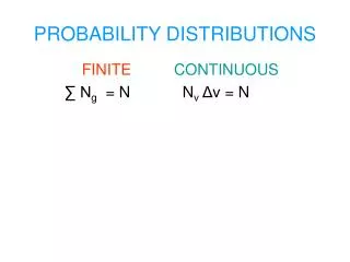
Probability distributions • We extend the probability analysis by considering random variables (usually the outcome of a probability experiment) • These (usually) have an associated probability distribution • Once we work out the relevant distribution, solving the problem is usually straightforward
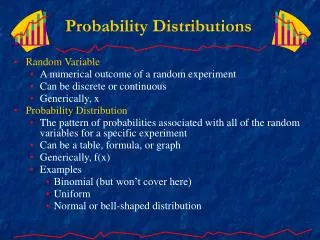
Random variables • Most statistics (e.g. the sample mean) are random variables • A random variable is a numeric event whose value is determined by a chance process or an experiment • The event should not be under the control of the observer; i.e., the value of the random variable is unknown before the experiment is carried out.
Random variables • Example 1: Suppose we roll two dice and take the sum of the numbers showing up. • This sum is clearly a random variable because its value is determined by chance • Such an experiment produces 11 possible values (what are they?) • Example 2: Consider a random experiment in which a coin is tossed three times. Let X be the number of heads. Let H represent the outcome of a head and T the outcome of a tail.
Random variables • The sample space for such an experiment will be: TTT, TTH, THT, THH, HTT, HTH, HHT, HHH. • Thus the possible values of X (number of heads) are x = 0,1,2,3. • Many random variables have well-known probability distributions associated with them. • To understand random variables, we need to know about probability distributions.
Discrete & continuous random variables • A discrete random variable is a variable that can assume only certain clearly separated values resulting from a count of some item of interest (countably finite or infinite). • Example: Let X be the number of heads when a coin is tossed 3 times. Here the values for X are x = 0,1,2,3. • A continuous random variable is a variable that can assume one of an infinitely large number of values. • Assumes any value within a designated range of values. • Example: Height of a student in this class.
Probability Distribution for Discrete RVs • Each value of a random variable has an associated probability • The probability distribution of a random variable lists all the possible values of the random variable and their corresponding probabilities • If P (X) is the probability that X is the value of the random variable, then
Discrete probability distributions • Suppose we toss a coin three times and want to observe the number of heads. • The possible values are 0, 1, 2, 3. • What is the probability distribution of the number of heads?
Expected value of discrete random variable • The mean of a random value is called its expected value • For discrete random variables, it is the weighted mean of all possible values of the random variable, with weights being the probabilities
Expected value • For the three tosses of a coin, we have • The expected value is not the value we “expect” on any single toss • Rather it is the long run average value (when the experiment is done a large number of times)
Variance for a random variable • The variance is given by • Or for computational ease, we use • Take square root to obtain standard deviation
Variance • = 3.0 – (1.5)2 = .75 • Standard deviation = .87
6-14 Practice • The Managing Director of Perfect Painters, a painting firm in Accra, has studied his records for the past 20 weeks and reports the following number of houses painted per week. Compute the mean and variance of the number of houses painted per week.
6-15 Solution • Probability Distribution:
6-16 Solution cont’d • Mean number of houses painted per week: • Variance of the number of houses painted per week:
Some standard probability distributions • Binomial distribution (discrete) • Normal distribution (continuous) • Poisson distribution (discrete)
When do they arise? • Binomial - when the underlying probability experiment has only two possible outcomes (e.g. tossing a coin) • Normal - when many small independent factors influence a variable (e.g. IQ, influenced by genes, diet, etc.) • Poisson - for rare events, when the probability of occurrence is low
The Binomial distribution • Applied when? • Only two mutually exclusive outcomes are possible in each trial (success or failure) • The outcomes in the series of trials are independent • The probability of success, denoted P, in each trial remains constant from trial to trial • The objective of using the BD is to determine the probability values for various possible number of successes (X), given the number of trails (n) and the known (and constant) probability of success (P)
The Binomial distribution • Consider five tosses of a coin. We can draw a tree diagram for this experiment, but we won’t. • Recall from last lecture, we can write the probability of 1 Head in 2 tosses as the probability of a head and a tail (in that order) times the number of possible orderings (# of times that event occurs). • P (1 Head) = ½ ½ 2C1 = ¼ 2 = ½ • We can apply same technique to calculate the probability for the number of heads in five tosses of a coin.
The Binomial distribution • P (X Heads in five tosses of a coin) • P(X= 0) = (½)0 (½)5 5C0 = 1/32 1 = 1/32 • P(X= 1) = (½)1 (½)4 5C1 = 1/32 5 = 5/32 • P(X= 2) = (½)2 (½)3 5C2 = 1/32 10 = 10/32 • P(X= 3) = (½)3 (½)2 5C3 = 1/32 10 = 10/32 • P(X= 4) = (½)4 (½)1 5C4 = 1/32 5 = 5/32 • P(X= 5) = (½)5 (½)0 5C5 = 1/32 1 = 1/32
Binomial distribution with different parameters • Eight tosses of an unfair coin (P = 1/6 )
The Binomial ‘family’ • Like other distributions, the Binomial is a family of distributions, members being distinguished by their different parameters. • The parameters of the Binomial are: • P - the probability of ‘success’ • n - the number of trials • Notation: X ~ B(n, P)
Formula for Calculating Binomial Probabilities • For the Binomial distribution, X ~ B(n, P), we can calculate the probability of X successes as P(X) = nCx *Px* (1-P)(n-x) • E.g. X ~ B(5, ½ ) means P(X) = 5Cx(½)x(1- ½)(5-x) and from this we can work out P(X) for any value of X.
Example • Probability of obtaining two heads in three tosses of a coin: X=2 and n=3 • X ~ B(3, ½ ) • P(X=2) = 3C2 (.5)2(.5) = 3×.25×.5 = .375 • Note that, nCX is the combination formula, which is equal to
Using complement rule • When the BD is used, it is typically because we wish to determine the probability or “X or more” successes [i.e., P(X ≥ xi)] or “ X or fewer successes [i.e., P (X ≤ xi)] • If the individual probabilities to be summed is large, it is easier to use the complement rule • Example: P (X ≥ xi) = 1 - P(X < xi)
Example • Suppose the probability is .05 that a randomly selected student of the University of Ghana owns a car. What is the probability of observing two or more student car-owners in a random sample of 20 students? • P(X≥2) = P(X=2) + P(X=3) + …..+ P(X=20) • P(X≥2) = 1 – P(X<2) = 1- P(X=0, 1) • = 1 – [P(X=0) +P(X=1)] • Now • P(X=0) = 20C0 (.05)0(.95)20 = .3585 • P(X=1) = 20C1 (.05)(.95)19 = .3774 • So P(X≥2) = 1 – (.3585 + .3774) = .2641
Mean and variance of the Binomial • Mean = E(X) = n P • Variance = σ2 = n P (1-P) • On average, you would expect 10 Heads from (n = ) 20 tosses of a fair (P = ½) coin (10 = 20 ½)
6-21 Practice • The Ministry of Employment reports that 20% of the labour force in Ghana is unemployed. From a sample of 14 members of the labour force, calculate the following probabilities using the formula for the binomial probability distribution: • three are unemployed • at least three are unemployed.
Solution • Three are unemployed: • P(x=3)=.250 • At least three are unemployed: • P(x ≥ 3) = 1 - P(x<3) • = 1 – [P(x=0) +P(x=1) + P(x=2)] • = 1- (.044 +.154 +.250) =.552
The Poisson distribution • It is a sampling process in which events occur over time or space. • The Poisson distribution is used to describe a number of processes or events such as • The distribution of telephone calls going through a switch board • The demand of patients for service at a health facility • The arrival of vehicles at a tollbooth • The number of accidents occurring at a road intersection, etc. • The Poisson is the limiting case of the Binomial when the probability of success is very small, i.e. BD becomes more and more skewed to the right as probability of success becomes smaller and smaller (rare events).
The Poisson distribution • Characteristics defining a Poisson random variable are • The experiment consists of counting the number of times a particular event occurs during a given time interval • The probability that the event occurs in one time interval is independent of the probability of the event occurring in another time interval • The mean number of events in each unit of time is proportional to the length of the time interval.
The Poisson distribution • The probability that the Poisson random variable will assume the value X is given by • For X = 0, 1, 2,3 ……. • λis the mean of the distribution (mean number of events occurring in a given unit of time) • e is approximately 2.7183 and is the base of the natural logarithms.
Example • Suppose an average of 2 calls per minute are received at a switchboard during a designated time interval, then the probability that exactly 3 calls are received in a randomly sampled minute is:
Poisson • As with the BD, the PD typically involves determining the probability of “X or more” or “X or fewer” number of events. • To calculate, we sum the appropriate probability values • The use of the complement rule may also come in handy • For example, we may want to calculate the probability of receiving 3 or more calls in a three-minute interval • That is P(X≥3) = P(X=3) + P(X=4) + …………… • Using the complement rule, we have • P(X≥3) = 1 - P(X<3) = 1 – [P(x=0) + P(x=1) + P(x=2)]
Poisson • From our proposition 3, we know the mean number of occurrences is proportional to the length of the time interval • So if we expect a mean of 2 calls per minute, in three minutes we must expect 6 calls • For an interval of 30 seconds, the mean number of calls is one • The probability of 5 calls in a three-minute interval implies λ = 6, so P(X=5 / λ=6) = .1606 • The probability of no calls in an interval of 30 seconds implies that λ = 1, so P(X=0 / λ=1) = .3679
Expected value and variance • The expected value and variance for a Poisson random variable are both equal to the mean number of events for the time interval of interest • E (X) = λ • Var (X) = λ
Poisson approximation of Binomial • When the probability of occurrence (success) is very small (P<.05) • And the number of trials is large (n>20) • So that λ = nP and we apply the Poisson formula • Some say use the Poisson in place of the Binomial when nP < 5
Example • A manufacturer claims a failure rate of 0.2% for its hard disk drives. In an assignment of 500 drives, what is the probability that, none are faulty, one is faulty, etc? • On average, 1 drive (0.2% of 500) should be faulty, so λ = nP = 1.
Example (continued) • The probability of no faulty drives is • The probability of one faulty drive is • and
