Download
1 / 53
530 likes | 534 Views
Meiosis, recombination fractions and genetic distance. Statistics 246, Spring 2004 Lecture 2A, January 22 Initially: pages 1-11. Later: pages 12-18. The action of interest to us happens around here : Chromosomes replicate , but stay joined at their centromeres Bivalents form

E N D
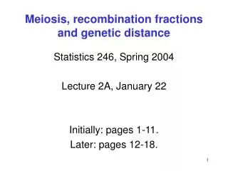
Meiosis, recombination fractions and genetic distance Statistics 246, Spring 2004 Lecture 2A, January 22 Initially: pages 1-11. Later: pages 12-18.
The action of interest to us happens around here : • Chromosomes replicate, but stay joined at their centromeres • Bivalents form • Chiasmata appear • Bivalents separate by attachment of centromeres to spindles. - the process which starts with a diploid cell having one set of maternal and one of paternal chromosomes, and ends up with four haploid cells, each of which has a single set of chromosomes, these being mosaics of the parental ones Source: http://www.accessexcellence.org
Four-strand bundle and exchanges (one chromosome arm depicted) sister chromatids sister chromatids 4-strand bundle (bivalent) 2 parental chromosomes Two exchanges 4 meiotic products
Chance aspects of meiosis • Number of exchanges along the 4-strand bundle • Positions of the exchanges • Strands involved in the exchanges • Spindle-centromere attachment at the 1st meiotic division • Spindle-centromere attachment at the 2nd meiotic division • Sampling of meiotic products • Deviations from randomness called interference.
A stochastic model for meiosis • A point process X for exchanges along the 4-strand bundle • A model for determining strand involvement in exchanges • A model for determining the outcomes of spindle-centromere attachments at both meiotic divisions • A sampling model for meiotic products • Random at all stages defines the no-interference or Poisson model.
A model for strand involvement • The standard “random” assumption here is • No Chromatid Interference(NCI): • each non-sister pair of chromatids is equally likely to be involved in each exchange, independently of the strands involved in other exchanges. • NCI fits the available data pretty well, but there are broader models.
The crossover process on meiotic products 1 change • Changes of (grand)parental origin along meiotic products are called crossovers. They form the crossover point processC along the single chromosomes. • Under NCI, C is a Bernoulli thinning of X with p=0.5, that is, each exchange has a probability of 1/2 of involving a given chromatid, independently of the involvement of other exchanges. 2 changes 1 change no change
From exchanges to crossovers • Usually we can’t observe exchanges, but on suitably marked chromosomes we can track crossovers. • Call a meiotic product recombinant across an interval J, and write R(J), if the (grand)parental origins of its endpoints differ, i.e. if an odd number of crossovers have occurred along J. Assays exist for determining whether this is so. We usually write pr(R(J))=r, and call r the recombination fraction. Recombination across the interval No recombination Recombination No recombination
Counting recombinants R and non-recombinants NR across the interval AB 4 NR 2R, 2NR 4NR 2R, 2NR 2R, 2NR 4R
Mather’s formula • Under NCI, if n>0, pr(R(J) | X(J) = n ) = 1/2. • Proof. Suppose that n>0. Consider a particular chromatid. It has a probability of 1/2 of being involved in any given exchange, and its involvement in any of the n separate exchanges are independent events. Thus the chance that it is involved in an odd number of exchanges is the sum over all odd k of the binomial probabilities b(k; n, 1/2), which equals 1/2 (check). • Corollary (Mather): pr(R(J)) = 1/2 pr( X(J) > 0). • It follows that under NCI, the recombination fractionr =pr(R(J)) is monotone increasing in the size of J, and ≤ 1/2.
The Poisson model • Suppose that the exchange process X is a Poisson process, i.e. that the numbers of exchanges in any pairwise disjoint set of intervals are mutually independent Poisson random variables. Denoting the mean number of exchanges in interval J by (J), we can make a monotone change of the chromosome length scale to convert this mean to |J|, where |J| is the length of J. This foreshadows the important notion of genetic or map distance, where rate = length. • Exercise: Prove that if X is a Poisson process, so is the crossover process C.
r12 r23 1 2 3 r13 r13 r12 + r23 Recombination and mapping • Sturtevant (1913) first used recombination fractions to order (i.e. map) genes. Problem: the recombination fraction does not define a metric. • Let’s consider 3 loci, denoted by 1, 2 and 3, and put rij = pr(R(i--j)). In general,
Triangle inequality • We will prove that under NCI, r13 ≤ r12 + r23. To see this, define • p00= pr(R(1--2)&R(2--3)), p01= pr(R(1--2)&R(2--3)) • p10= pr(R(1--2)&R(2--3)), p11= pr(R(1--2)&R(2--3)), • where the denotes the complement (negation) of the event. • Now notice that • R(1--2)&R(2--3) + R(1--2)&R(2--3) = R(1--2), • R(1--2)&R(2--3) + R(1--2)&R(2--3) = R(2--3), and • R(1--2)&R(2--3) + R(1--2)&R(2--3) = R(1--3) (think about this one). • Thus we have • p10 + p11 = r12 ,p01 + p11 = r23 , and p00 +p11 = 1-r13 . • Adding the three equations, and using the fact that the pij sum to 1 gives • r12 + r23 - r13 = 2p11 ≥ 0. • In general this inequality is strict. Under the Poisson model, p11 = r12r23 .
d12 d23 1 2 3 d13 d13 = d12 + d23 Map distance and mapping Map distance: d12 = E{C(1--2)} = av # COs in 1--2 Unit: Morgan, or centiMorgan. • Genetic mapping or applied meiosis: a BIG business • Placing genes and other markers along chromosomes; • Ordering them in relation to one another; • Assigning map distances to pairs, and then globally.
Haldane’s map function • Suppose that X is a Poisson process, and that the map length of an interval J is d. • Then the mean number (J) of exchanges across J is 2d, and by Mather, the recombination fraction across J is • More generally, map functions relate recombination fraction to genetic distance; r ~ d for r small.
The program from now on • With these preliminaries, we turn now to the data and models in the literature which throw light on the chance aspects of meiosis. • Mendel’s law of segregation: a result of random sampling of meiotic products, with allele (variant) pairs generally segregating in precisely equal numbers. • As usual in biology, there are exceptions.
Randomspindle-centromere attachment at 1st meiotic division x smaller In 300 meioses in an grasshopper heterozygous for an inequality in the size of one of its chromosomes, the smaller of the two chromosomes moved with the single X 146 times, while the larger did so 154 times. Carothers, 1913. larger
Tetrads • In some organisms - fungi, molds, yeasts - all four products of an individual meiosis can be recovered together in what is known as an ascus. These are called tetrads. The four ascospores can be typed individually. • In some cases - e.g. N. crassa, the red breadmold - there has been one further mitotic division, but the resulting octads are ordered.
Using ordered tetrads to study meiosis • Data from ordered tetrads tell us a lot about meiosis. For example, we can see clear evidence of 1st and 2nd division segregation. • We first learned definitively that normal exchanges occur at the 4-stand stage using data from N. crassa, and we can also see that random spindle-centromere attachment is the case for this organism. • Finally, aberrant segregations can occasionally be observed in octads.
Different 2nd division segregation patterns Under random spindle-centromere attachment, all four patterns should be equally frequent.
2-strand double exchanges lead to FDS There is a nice connexion between the frequencies of multiple exchanges between a locus and its centromere and the frequency of 2nd division segregations at that locus.
A simple calculation and result • Let Fk (resp. Sk) denote the number of strand-choice configurations for k exchanges leading to first (resp. second) division segregation at a segregating locus. By simple counting we find • F0 =1 and So= 0, while for k>0, • Fk+1 = 2Sk , and Sk+1 = 4Fk + 2Sk . • Assuming NCI, the proportion sk of second-division segregants among meioses having k exchanges between our locus and the centromere is
If the distribution of the # of exchanges is (xk), then the frequency of SDSs is If the distribution is Poisson (2d) then we find This is a map-function: between the unobservable map distance d and the observable SDS frequency s.
Interference: the state of play • Total number of exchanges on an arm rarely Poisson • Positions of exchanges rarely Poisson in map distance (i.e. crossover interference is the norm) • Strand involvement generally random (i.e. chromatid interference is rare) • Spindle-centromere attachment generally random (non-random attachments are quite rare) • The biological basis for crossover interference is only slowly becoming revealed; stay tuned.
1 2 3 The Poisson model implies independence of recombination across disjoint intervals pr(R(1--2) & R(2--3)) = pr(R(1--2)) pr(R(2--3))
I II ec cv sc Morgan’s D. melanogaster data (1935) 0: no recombination; 1: recombination 0 1 0 13670 824 1 1636 6* *the number of double recombinants that we would expect if recombination events across the two intervals were independent is 85 Clearly there are many fewer double recombinants than the independence model would predict. This phenomenon is called crossover interference..
2 3 1 4 A measure of crossover interference The coincidence coefficient S4 for 1--2 & 3--4 is: pr(R(1--2) & R(3--4)) pr(R(1--2)) pr(R(3--4)) = pr(R(1--2) | R(3--4)) pr(R(1--2)) No crossover interference (for these intervals) if S4= 1 Positive interference (inhibition) if S4 < 1.
An observation concerning crossover interference • The coefficient S4 for short disjoint intervals, begins at zero with zero cM separation for Drosophila and Neurospora, and reaches unity at about 40 cM in both organisms, despite the fact that the crossover rate per kb is about ten times higher in N. crassa than in D. melanogaster. • Thus interference somehow follows map distance more than it does the DNA bp. • There are a number of other intriguing observations like this concerning interference.
Stochastic models for exchanges • Count-location models • Renewal process models • Other special models, including a polymerization model
Count-Location Models Barrett et al (1954), Karlin & Liberman (1979) and Risch & Lange(1979) These models recognize that interference influences distribution of the number of exchanges, but fail to recognize that the distance between them is relevant to interference, which limits their usefulness. N = # exchanges along the bivalent. (1) Count distribution: qn = P(N = n) (2) Location distribution: individual exchanges are located independently along the four-strand bundle according to some common distribution F. Map distance over [a, b] is d = [F(b) – F(a)]/2, where = E(N).
Cx Co Cx Co Cx Co X X X X X X C C C C C C The Chi-Square Model Fisher et al (1947), Cobbs (1978), Stam (1979), Foss et al (1993), Zhao et al (1995) Modeling exchanges along the 4-strand bundle as events from a stationary renewal process whose inter-event distribution is 2 with an even number of degrees of freedom. The x events are randomly distributed and every (m+1)st gives an exchange: m=1 below. The chi-square model is denoted by Cx(Co)m. m = 0 corresponds to the Poisson model.
Evidence in support of the chi-squared model, I • The model fit the Drosophila data by embodying two conspicuous features of those data: the curve for S4 vs linkage map distance had a toe of the right size and reached a maximum a little short of the mean distance between exchanges.
Coincidence here means S4 ; the data are from 8 intervals along the X chromosome of D. melanogaster, 16,136 meioses, Morgan et al (1935) McPeek et uno (1995)
Evidence in support of the chi-squared model, II • The model predicts multilocus recombinationdata in a variety of organisms pretty well, typically much better than other models • The model fits human crossover location data pretty well too, both in frequency and distribution of location.
Model comparisons using Drosophila data McPeek et uno (1995)
Human Broman &Weber, 2000
Biological interpretation of the chi-squared or Cx(Co)m model • The biological interpretation of the chi-squared model given in Foss, Lande, Stahl, and Steinberg 1993, is embodied in the notation Cx(Co)m : the C events are crossover initiation events, and these resolve into either reciprocal exchange events Cx, or gene conversions Co, in a fairly regular way: crossovers are separated by an organism-specific number m of conversions. • In some organisms the relative frequency of crossover associated and non-crossover associated conversion events can be observed. • Question: who’s counting?
Fitting the Chi-square Model to Various Organisms Gamete data: D. melanogaster: m = 4 Mouse: m = 6 Tetrad data: N. crassa: m = 2 S. cerevisiae: m = 0 - 3 (mostly 1) S. pombe: m = 0 Pedigree data: Human (CEPH): m = 4 The chi-square model has been extremely successful in fitting data from a wide variety of organisms rather well.
Failure of the Cx(Co)m model with yeast • The biological interpretation of the chi-squared model embodied in the notation Cx(Co)m is that crossovers are separated by an organism-specific number of potential conversion events without associated crossovers. • It predicts that close double crossovers should be enriched with conversion events that themselves are not associated with crossovers. • With yeast, this prediction can be tested with suitably marked chromosomes. • It was so tested in Foss and Stahl, 1995 and failed.
Very brief summary of some current research on recombination • It appears that many organisms have two meiotic recombination pathways, one of which lacks interference. There the protein MSH4 binds to recombinational intermediates and directs their resolution as Cx’s, while in its absence these resolve as Co’s. The intermediates seem to be brought into clusters, called late recombination nodules, and MSH4 binds to one member per cluster, e.g. the middle one. This resolves as a crossover while the others resolve as noncrossovers, leading to the “counting model”.
Challenges in the statistical study of meiosis Understanding the underlying biology Combinatorics: enumerating patterns Devising models for the observed phenomena Analysing single spore and tetrad data, especially multilocus data Analysing crossover data
Acknowledgements • Mary Sara McPeek, Chicago • Hongyu Zhao, Yale • Karl Broman, Johns Hopkins • Franklin Stahl, Oregon
References • www.netspace.org/MendelWeb • HLK Whitehouse: Towards an Understanding of the Mechanism of Heredity, 3rd ed. 1973 • Kenneth Lange: Mathematical and statistical methods for genetic analysis, Springer 1997 • Elizabeth A Thompson Statistical inference from genetic data on pedigrees, CBMS, IMS, 2000.