Download

1 / 23
230 likes | 281 Views
This module explores joint distributions of random variables and the concept of independence in probability and statistics, covering joint distribution of discrete and continuous random variables, marginal distributions, and tests for independence. Examples and exercises are provided to enhance understanding.

E N D
CIS 2033 based onDekking et al. A Modern Introduction to Probability and Statistics. 2007Slides by Michael Maurizi Instructor Longin Jan Latecki C9: Joint Distributions and Independence
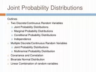
9.1 – Joint Distributions of Discrete Random Variables • Joint Distribution: the combined distribution of two or more random variables defined on the same sample space Ω • Joint Distribution of two discrete random variables:The joint distribution of two discrete random variables X and Y can be obtained by using the probabilities of all possible values of the pair (X,Y) Joint Probability Mass function p of two discrete random variables X and Y: Joint Distribution function F of two random variables X and Y: Can be thought of as the sum of the elements in box it makes with the upper-left corner.
9.1 – Joint Distributions of Discrete Random Variables Example: Joint Distribution of S and M. S = The sum of two dice, M = The maximum of two dice. Quick exercise 9.1 List the elements of the event {S = 7,M = 4} and compute its probability.
9.1 – Joint Distributions of Discrete Random Variables Example: Joint Distribution of S and M. S = The sum of two dice, M = The maximum of two dice. Quick exercise 9.1 List the elements of the event {S = 7,M = 4} and compute its probability. The only possibilities with the sum equal to 7 and the maximum equal to 4 are the combinations (3, 4) and (4, 3). They both have probability 1/36, so that P(S = 7,M = 4) = 2/36.
9.1 – Marginal Distributions of Discrete Random Variables • Marginal Distribution: Obtained by adding up the rows or columns of a joint probability mass function table. Literally written in the margins. • Let p(a,b) be a joint pmf of RVs S and M. The marginal pmfs are then given by Example: Joint Distribution of S and M. S = The sum of two dice, M = The maximum of two dice.
9.1 – Joint Distributions of Discrete Random Variables: Examples Example: Joint Distribution of S and M. S = The sum of two dice, M = The maximum of two dice. Compute joint distribution function F(5, 3).
9.4 – Independent Random Variables Tests for Independence: Two random variables X and Y are independent if and only if every event involving X is independent of every event involving Y.
Example 3.6 (Baron book) • A program consists of two modules. The number of errors, X, in the first module and the number of errors, Y, in the second module have the joint distribution, P(0, 0) = P(0, 1) = P(1, 0) = 0.2, P(1, 1) = P(1, 2) = P(1, 3) = 0.1, P(0, 2) = P(0, 3) = 0.05. Find (a) the marginal distributions of X and Y, (b) the probability of no errors in the first module, and (c) the distribution of the total number of errors in the program. Also, (d) find out if errors in the two modules occur independently.
Table 4.2: (Baron book) • Joint and marginal distributions in discrete and continuous cases.
9.2 – Joint Distributions of Continuous Random Variables • Joint Continuous Distribution: Like an ordinary continuous random variable, only works for a range of values. There must exist a function f that fulfills the following properties for there to be a joint continuous distribution: Marginal distribution function of X: Marginal distribution function of Y:
9.2 – Joint Distributions of Continuous Random Variables Joint distribution function: F(a,b) can be constructed given f(x,y), and vice versa Marginal probability density function: You need to integrate out the unwanted random variable to get the marginal distribution.
We can also determine fY(y) directly from f(x,y) (Quick Exercise 9.5). For y between 1 and 2:
9.3 – More than Two Random Variables Assuming we have n random variables X1, X2, X3, … Xn. We can get the joint distribution function and the joint probability mass functions.
9.4 – Independent Random Variables Tests for Independence of more than two random variables.
9.5 – Propagation of Independence Independence after a change of variable: If a function is applied to several independent random variables, the new resulting random variables will also be independent.