Download

1 / 25
270 likes | 384 Views
Explore deep learning models for bacterial taxonomy using convolutional neural networks and deep belief networks on 16S rRNA data.

E N D
Deep learning models for bacteria taxonomic classification of metagenomics data Antonino Fiannaca1, Laura La Paglia2, Massimo La Rosa2, Giosue Lo Bosco3, Giovanni Renda4, Riccardo Rizzo2, Salvatore Gaglio2,4, and Alfonso Urso2 1CNR-ICAR, National Research Council of Italy, Via Ugo La Malfa, 153, Palermo, Italy 2CNR-ICAR, National Research Council of Italy, Via Ugo La Malfa, 153, Palermo, Italy 3Dipartimento di Matematica e Informatica, Università degli studi di Palermo, Via Archirafi, 34, Palermo, Italy 4Dipartimento dell'Innovazione Industriale e Digitale, Università degli studi di Palermo, Viale Delle Scienze, ed.6, Palermo, Italy Published in BMC Bioinformatics, 19:198, 2018 Presenter: Wei Chun Chen (John)
Why do we study metagenomics? • Metagenomics is the study of genetics of microorganisms such as bacteria, virus, protozoa, fungi, and algae • Essential components of life on earth • Bacteria: benefits and adversaries
Classification of bacteria genomes • A common approach for profiling the bacterial communities is to conduct comparative analysis of ribosomal RNA sequences (rRNA), specifically the 16S ribosomal RNA. • 16S rRNA gene is considered mostly highly conserved between different species of bacteria, and it’s a standard marker gene for bacterial classification. • 16S rRNA gene does also contain several hypervariable regions (V1-V9), which can provide maximum discriminating power to identify different bacterial groups. 16S rRNA
Classification of bacteria genomes • Next Generation Sequencing (NGS) technologies are used for 16S rRNA sequencing. • (1) Whole Genome Shotgun (or 16S shotgun (SG)) is used to obtain the full-length 16S rRNA genes. • (2) Amplicon (AMP) is used to obtain only the specific hypervariable region (V3-V4) of the 16S rRNA genes.
Related Work • Pervious studies on metagenomics focused on the use of machine learning methods. • Taxonomic profiling based on alignment and assembly of the whole genome sequences suffered from computational issues such as time complexities. • Most of deep learning implementation are focused in genomic medicine and medical imaging research, but not in metagenomics.
Objective • To this end, the goal of this study is to classify bacterial sequences (from SG and AMP dataset) using the two deep learning models: convolutional neural network and deep belief network.
Methodology Figure 1. Proposed training process. Starting from 16S reads, we proposed a vector representation and a deep learning architecture to obtain trained models for taxonomic classification.
Methodology • Generate 16S rRNA dataset • Generate SG and AMP dataset • Short-reads representation (k-mers co-occurrence) • CNN network • Deep Belief network • RDP (ribosomal database project) classifier as reference (naïve Bayesian classifier)
Generate 16S rRNA dataset • First, using the bioinformatics tool REAGO, conduct homology search to identify reads from the original 16S rRNA gene. • Then, assemble the reads into the full-length genes. • Of the 57,788 16S rRNA gene sequences, randomly select 1,000 sequences belonging to the proteobacteria phylum. • The simulated dataset contains 100 genera, and 10 species from each genus. Yuan et al., Bioinformatics, 2015
Generate Short-reads SG and AMP dataset • Each library (dataset) contains about 28,000 short-reads (about 28 reads per sequence). Angly et al., Nucleic Acids Research, 2012
Short-reads representation (k-mers) k = 4, stride = 1 ACCAGTT ACCA
Short-reads representation (k-mers) k = 4, stride = 1 ACCAGTT ACCA CCAG
Short-reads representation (k-mers) k = 4, stride = 1 ACCAGTT ACCA CCAG CAGT
Short-reads representation (k-mers) k = 4, stride = 1 ACCAGTT ACCA CCAG k-mer frequency vector (input vector length = 4k) CAGT AGTT
Figure 2. The dataset characteristics. The graph shows the mean length of sequences of 0’s and the mean length of sequences of npn-0’s values for each value of K, where K is the order of the K-mer.
Figure 3. The convolutional neural network. The architecture of the convolutional neural network used. Here, L represents the dimension of the input vector x, L = 4K were K is the dimension of the K-mers. In the upper part of the figure the representation of the C1 convolutional-maxpooling layer, where K stands for kernel size and n1 is the number of kernels. The block M1 represents the set of weights for the connections from input to hidden layer, the block M2 represents the weighted connections from hidden layer to output. y is the CNN output. Relu
Figure 4. CNN kernel size configuration. Classification scores at varying of CNN kernel sizes at genus level for both (a) SG and (b) AMP. Accuracy = (TN + TP) / (TN + TP + FN + FP) Precision = TP / (TP + FP) Recall = TP / (TP + FN) • The accuracy and precision of the AMP dataset are more resistant to fluctuation as kernel size changes.
Figure 5. Configuration of CNN kernel numbers. Classification scores at varying of CNN number of kernels at genus level for both (a) SG and (b) AMP. • The accuracy and precision of the AMP dataset are more resistant to fluctuation as number of kernel changes.
Figure 6. The deep belief network. An example of deep belief network with two RBM layers for binary classification. In this figure, L represents the dimension of the input vector x, whereas, h and w represent the hidden units and the weights of each RBM respectively. y is the binary output. RBM, Restricted Boltzmann Machines.
Figure 7. Accuracy validation of CNN classifier, according to k-mer size. Classification of (a) SG and (b) AMP datasets with CNN architecture. • Accuracy increases as k increases. • Higher accuracy is shown using AMP dataset.
Figure 8. Accuracy validation of DBN classifier, according to k-mer size. Classification of (a) SG and (b) AMP datasets with DBN architecture. • DBN has a more stable growing trend.
Figure 9. Accuracy validation of CNN, DBN, RDP classifier, at genus level. Comparison among CNN, DBN, and RBN classification algorithms, with respect to (a) SG and (b) AMP datasets. 85% 81% 80% • Using the AMP dataset, in term of accuracy, CNN and DBN provide higher scores than those using the SG dataset. 91% 91% 83%
Summary • Performance of the classifiers applied to the AMP dataset (focused on the hypervariable regions of 16S rRNA) is better than the SG dataset (entire 16S rRNA sequences). • The CNN and DBN achieved higher scores than the RDP classifier. • Future study will aim to combine both deep learning networks to improve metagenomics classification performance.