Download
1 / 1
10 likes | 160 Views
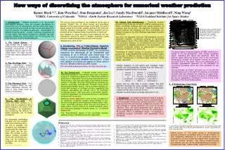
This study explores new approaches to discretizing the three-dimensional atmosphere and addressing the complexities of numerical weather prediction. Traditional lat-lon grid methods encounter singularities at poles, prompting the adoption of alternative grids such as cubed sphere, Yin-Yang, Fibonacci, and icosahedral grids. We introduce the Finite-Volume, Flow-Following, Icosahedral Model (FIM), which features advanced mass transfer algorithms and maintains isentropic conditions through vertical grid hybridization. This innovative modeling framework aims to improve forecasting accuracy by overcoming traditional grid limitations.

E N D
Vertical migration of grid points and interlayer mass transfer are simultaneously inferred from the mass con-servation equation written in the form where only the right side is known initially. The ALE algorithm provides the extra condition needed to deter-mine the two terms on the left [2]. Traditional hydrostatic models set first term on the left to zero. (Related non-ALE hybrid coordinate work: [5,6,11,13].) New ways of discretizing the atmosphere for numerical weather prediction Rainer Bleck1,2,3, Jian-Wen Bao2, Stan Benjamin2, Jin Lee2, Sandy MacDonald2, Jacques Middlecoff2, Ning Wang21CIRES, University of Colorado 2NOAA - Earth System Research Laboratory 3NASA Goddard Institute for Space Studies The severe 2-pole problem in the traditional lat-lon grid is thereby “diluted” into 12 rather benign grid anomalies. Because of the near-circular shape of grid cells, this grid is ideally suited for the finite volume approach [7] where dif-ferential operators (divergence, vorticity, gradient) are ex-pressed as line integrals along the perimeter of a grid cell. One obstacle to using this grid is that traditional 2-D dis-cretizations cannot be used. A weather prediction model using an icosahedral grid must be built from scratch. (Related work: [8,9,10,12]) 6b. Vertical Grid Hybridization – Coordinate surface-ground intersections are avoided in FIM by combining isen-tropic coordinate surfaces aloft with terrain-following () surfaces near the ground. The algorithm managing inter-actions between the isentropic and the -coordinate sub-domain is based on the ALE (Arbitrary Lagrangian-Eulerian) scheme [4]. Like ALE, the algorithm built into FIM maintains non-zero separation between coordinates surfaces by transferring mass between layers. This unfortunately makes layers lose their isentropic character. To counteract this trend, which is exacerbated by diabatic processes in the atmosphere, our algorithm continually checks for opportunities to restore isentropic conditions in a layer [1,3]. Restoration of “target” entropy (or its proxy, potential tem-perature ) is accomplished by entraining air from a neigh-boring layer of different entropy. In determining the rate of transfer, maintenance of minimum layer thickness trumps “target” restoration. 1. Introduction – Weather prediction is an agonizingly multi-faceted problem. Here we consider alternatives for discretizing the 3-D atmosphere and the differential equa-tions governing its evolution so they can be accurately sol-ved on a sphere. The traditional approach - discretization in latitude-longitude space - creates numerical singularities at the two poles. Alternatives proposed to alleviate the pole problem include the cubed sphere, the Yin-Yang grid, the Fibonacci grid, and the icosahedral grid. Meridional vertical section through the model atmosphere, showing coordinate surfaces (solid lines), wind speed (m/s, shaded contours), and (0K, color). Ordinate: pressure (hPa) 2. The Cubed Sphere – A cube turned into a sphere by inflating it like a balloon. Popular because conventional x,y dis-cretizations can be used on indi-vidual faces. The eight corners of the cube require special treat-ment. (Picture credit: J. W. Hernlund, P. J. Tackey, Comp. Fluid Solid Mech., 2003) 6. Introducing FIM, a “Finite-Volume, Flow-Fol-lowing, Icosahedral” Weather Prediction Model – In FIM, recently developed at ESRL, the underlying equations are discretized on an icosahedral grid consisting of up to 655,000 cells (mesh size ~30 km). In a second break with convention, FIM fea-tures a nonstandard vertical discretization. Cloud and radiation processes are based on those used in the U.S. Weather Service’s GFS model. For more detailed documentation, see http://fim.noaa.gov. The above figure illustrates aspects of FIM’s vertical coor-dinate. In the free atmosphere, color follows coordinate layers, indicating that layers are isentropic. Near the ground, layers follow the terrain. Due to the north-south temperature contrast, the domain extends up higher in the south than in the north. This is not unwelcome as it provides “guaranteed” resolution for the simulation of convective processes which are more prevalent at low latitudes. Two jet streams are shown: the polar one on the left and the subtropical one on the right. The packing of isentropes beneath both jets indicates the presence of upper-tropo-spheric fronts which represent extrusions of stratospheric air into the troposphere. Simulation of fronts is one of the strengths of the coordinate system. 3. The Yin-Yang Grid –Two pieces resembling cupped hands pressed together to form an enclosure. Conventional x,y discretizations can be used, but information transfer between the Yin and the Yang grid requires overlaps and interpolation. (Picture credit: Takahashi etal., Proc. 7th Int. Conf. HPCAsia’04) 6a. The Vertical Grid – Computer models cannot solve differential equations; they actually solve sets of algebraic equations. Substituting algebraic for differential equations gives rise to “dispersion” errors during horizontal and ver-tical transport. One can hide these errors behind a smoke screen of naturally occurring mixing/stirring processes by aligning coordinate surfaces with surfaces along which stirring preferentially occurs. These surfaces typically co-incide with surfaces of constant entropy, suggesting that transport calculations be carried out in an isentropic coordinate system. FIM uses such a coordinate system, modified (“hybridized”) to avoid intersections of coordinate surfaces with the ground. Reducing lateraldispersion errors is only one aspect of an isentropic coordinate system. Since entropy is con-served during gravity wave-induced vertical motion, isen-tropic coordinate surfaces follow the ups and downs of wave motion. Hence, there is no vertical interlayer trans-port during the passage of gravity waves, i.e., no verticaldispersion. The “flow-following” aspect of the coordinate requires spacing of layer interfaces to be time-dependent. 4. The Fibonacci Grid – Grid point locations mimic the way nature distributes discrete ob-jects in finite areas (such as seeds in seed pods). (Picture credit: Swinbank and Purser 2005) 8. A Rudimentary Case Study 7. Drawbacks – No weather prediction model is superior to others in all possible respects. Known shortcomings of the coordinate include poor vertical resolution in unstra-tified (constant-) and thermally unstable air columns. Ab-rupt changes in vertical resolution can occur at the interface. Time- and space-dependent layer spacing re-quires sophisticated transport schemes for conservation. At present, FIM is a hydrostatic model – a handicap in simulating buoyant convection and associated cloud processes. 5. The Icosahedral or “Soccer Ball” Grid – The black and white patches on a soccer ball are created by fitting white hexagons into each of the 20 triangles in an icosahedron and combining the leftover tri-angle fragments into 12 black pentagons. By repeatedly subdividing triangles into four smaller ones and combining the fi-nal set of triangles into hexagons and pentagons, honeycomb-like high-reso-lution grids can be cre-ated. The number of pen-tagons remains constant during the refinement pro-cess, but the number of hexagons can be arbitra-rily large. (Picture credit: G.Grell, NOAA-ESRL) References Benjamin, S.G., G.A. Grell, J.M. Brown,T.G. Smirnova and R. Bleck, 2004: Mesoscale weather prediction with the RUC hybrid isentropic-terrain-following coordinate model. Mon. Wea. Rev., 132, 473-494. Bleck, R., 1978: On the use of hybrid vertical coordinates in numerical weather prediction models. Mon. Wea. Rev., 106, 1233-1244, Bleck, R., 2002: An oceanic general circulation model framed in hybrid isopycnic-Cartesian coordinates. Ocean Modelling, 4, 55-88, Hirt, C. W., A. A. Amsden, and J. L. Cook, 1974: An arbitrary Lagrangian-Eulerian computing method for all flow speeds, J. Comput. Phys., 14, 227-253. Johnson, R. D.,T. H. Zapotocny, F. M. Reames, B. J. Wolf, and R. B. Pierce, 1993: A comparison of simulated precipitation by hybrid isentropic-sigma and sigma models, Mon. Wea. Rev., 121, 2088-2114. Konor, C. S. and A. Arakawa, 1997: Design of an atmospheric model based on a generalized vertical coordinate. Mon. Wea. Rev., 125, 1649-1673. Lin, S. J., 2004: A vertically Lagrangian finite-volume dynamical core for global models. Mon. Wea. Rev.,132, 2293-2307. Majewski, D., D. Liermann, P. Prohl, B. Ritter, M. Buchhold, T. Hanisch, G. Paul, and W. Wergen, 2002: The operational global icosahedral-hexagonal gridpoint model GME: Description and high-resolution tests, Mon. Wea. Rev., 130, 319—338. Sadourny, R., A. Arakawa, and Y. Mintz, 1968: Integration of the non-divergent barotropic vorticity equation with an icosahedral-hexagonal grid for the sphere. Mon. Wea. Rev., 96, 351-356. Tomita, H.,M. Tsugawa, M. Satoh, and K. Goto, 2001: Shallow water model on a modified icosahedral geodesic grid by using spring dynamics. J. Comput. Phys., 174, 579-613. Webster, S., J. Thuburn, B. J. Hoskins, and M. J. Rodwell, 1999: Further development of a hybrid-isentropic GCM, Quart. J. Roy. Meteorol. Soc., 125, 2305-2331. Williamson, D. L., 1968: Integration of the barotropic vorticity equation on a spherical geodesic grid. Tellus, 20, 642-653. Zapotocny, T.H., D. Johnson, and F.M. Reames, 1994: Development and initial test of the University of Wisconsin global isentropic-sigma model. Mon. Wea. Rev., 122, 2160-2178. 5- and 2.5-day (left/right) precipitation forecasts for the 12-hr period ending 1200 GMT, 14 March 2008, from FIM and GFS (top/bottom). Caution: map projections, units, color bars differ. Salient points: (1) The phase speed of rain-producing synoptic systems is remarkably close in the two models. (2) One noteworthy difference is in the predicted extent of precipitation over the central Gulf states. Both models stray from the “perfect” forecast – two distinct rainfall maxima, one offshore and one on the Arkansas-Missouri border. In this particular case, neither model outperforms the other.