Download
1 / 55
570 likes | 599 Views
Metabolic networks. John Pinney Theoretical Systems Biology group j.pinney@imperial.ac.uk. 341 Introduction to Bioinformatics: Biological Networks 25th February 2010. Part 1: Constructing metabolic networks. What is metabolism?.

E N D
Metabolic networks John Pinney Theoretical Systems Biology group j.pinney@imperial.ac.uk 341 Introduction to Bioinformatics: Biological Networks 25th February 2010
What is metabolism? • “Metabolism is the set of chemical reactions that occur in living organisms in order to maintain life.” Image: section through an Escherichia coli cell by David Goodsell
What is metabolism? • Key classes of biochemicals: • amino acids • proteins • carbohydrates • bacterial envelope • nucleotides • genetic material • lipids • membranes • coenzymes • transfer chemical groups • minerals • assist in biochemical transformations
Enzymes • Metabolic reactions are catalysed by proteins called enzymes. glucose glucose 6-phosphate
Metabolic pathways • Traditionally, biochemists consider a series of consecutive metabolic reactions to form a pathway. Image: CK12.org
Metabolic networks • However, pathways often overlap so much that it is more accurate to consider the set of all metabolic reactions as forming a network. Image: Wikipedia
How should we represent metabolic networks? • Traditional textbook representation: • Compounds are shown as boxes. • Arrows connect compounds to show interconversions. • Arrows are labelled with the name of the associated enzyme. • Cofactors (commonly-used compounds) included with curved arrows. Image: Michal, G. (1993). Biochemical Pathways Poster. Boehringer Mannheim GmbH
Why should we study metabolic networks? • Fundamental to life • Since enzymes are encoded in the genome, metabolism is one mechanism by which an organism’s genotype (specific set of genes) is connected to its phenotype (how it behaves). Many metabolic processes are common to all forms of life. • Biotechnology • Deep understanding of the metabolic networks of bacteria is needed if they are to be genetically modified to produce a desired product with maximum yields. • Medicine • Aberrations in human metabolism are fundamental to diseases such as diabetes and some types of cancer. • Knowledge of the metabolic networks of pathogens and parasites can help to select drug targets (or target combinations) that will be most effective.
How should we represent metabolic networks? • Traditional textbook representation: • Compounds are shown as boxes. • Arrows connect compounds to show interconversions. • Arrows are labelled with the name of the associated enzyme. • Cofactors (commonly-used compounds) included with curved arrows. Image: Michal, G. (1993). Biochemical Pathways Poster. Boehringer Mannheim GmbH
Representing metabolic networks for systems biology • simple graph • metabolite digraph bipartite digraph reaction or more complex still..? enzyme
Metabolic reconstruction • Task: • Given the genome sequence for an organism, find its metabolic network. Resources: Sequence databases Genome annotations Databases of metabolic reactions Tools: Sequence similarity searches Text extraction Machine learning Experimental data (high- and low-throughput) Francke Cet al. (2005)
Metabolic reconstruction from a genome annotation • For well-studied organisms, a great deal of information about metabolism is already known. • Genome annotations label each gene with our current knowledge. • Enzymatic functions are often described in such annotations using the E.C. (Enzyme Commission) hierarchical numbering system. EC 5.3.1.9 glucose-6-phosphate isomerase => isomerase 5.3 => intramolecular oxidorecuctases 5.3.1 => interconverting aldoses and ketoses
Metabolic reconstruction from a genome annotation • Once a set of enzymes has been collected, they can simply be projected onto a database of all known metabolic reactions to give a “first-pass” network reconstruction. • e.g. glycolysis / gluconeogenesis for chicken, Gallus gallus, taken from KEGG (Kyoto Encyclopedia of Genes and Genomes) • www.genome.jp/kegg
Metabolic reconstruction from a proteome • Often a well-curated genome annotation is unavailable, but we have a good idea of where the protein-coding genes are on the genome so can extract a predicted proteome (set of all protein sequences encoded by the genome). • The task is now to assign enzymatic functions to these protein sequences. genome sequence with known protein-coding regions. predicted proteins
annotated proteome new proteome Functional assignment by sequence similarity (e.g. BLAST) Metabolic reconstruction from a proteome • If a closely-related organism has a good annotation, it may be possible to identify orthologous (i.e. functionally equivalent) proteins using basic sequence alignment methods such as BLAST. • More sophisticated methods for orthology assignment are also available.
Metabolic reconstruction from a proteome • However, using profile models for enzyme domains is a more sensitive way to detect sequence similarities, especially across large evolutionary distances. Highly-conserved amino acids multiple alignment of enzyme domains from many species profile model (position-specific scoring matrix / profile HMM) library of models for all enzyme functions with known sequences
Metabolic reconstruction from a proteome Known ligand-binding residues from bacterial structure EPSP synthase ATP/GTP binding motif shikimate kinase McConkey GA et al. (2004)
Limitations of sequence-based methods • Large evolutionary distances • Transfer of function from a distant sequence may not be reliable. • Enzyme may be too divergent to be recognised from sequence. • Multiple functions • Some enzymes have multiple protein domains that have different functions. • An enzyme may “moonlight” - i.e. catalyse several different reactions using the same active site. • Reactions with unknown sequences • There are several known metabolic reactions for which no example enzyme sequences are known. • Unknown reactions • Across all kingdoms of life, there are many hundreds of metabolic reactions that are as yet completely uncharacterised!
Manual curation • Computational assignment of gene function is not 100% accurate! • It will always be important to examine and refine initial automated metabolic reconstructions carefully before attempting to analyse the resulting network. • Comparative genomics can be a powerful tool in network curation. • By comparing genomes between different species, we attempt to use their shared evolutionary histories to help us identify gene functions more accurately. • What genes are close to this gene? • Has this gene ever fused with another one? • Which genes tend to be present in the same organisms as this one? • Which genes control whether this one is switched on? • What experimental evidence is there?
consumed but not produced intermediate reaction missing produced but not consumed Gaps in a reconstructed network • Even after curation, a network may still contain obvious gaps, also known as pathway holes. source sink
shared pattern anticorrelated pattern Methods for gap-filling • Phylogenetic profiling (evidence for functionally associated genes) • Anticorrelation analysis (evidence for functionally analogous genes) gene ? species ? Osterman A and Overbeek R (2003); Pellegrini M et al. (1999)
Methods for gap-filling • Evidence from various sources can be integrated using machine learning to give an overall likelihood that a particular gene might fill a particular pathway hole. • For parasitic or symbiotic organisms, we also need to consider the possibility of metabolite exchange with the host or subversion of host enzymes. Green ML et al. (2004)
Analysis of metabolic networks • Metabolic networks can be analysed on several different levels. • Topologically • Basic network structure • Stoichiometrically • Considering the numbers of molecules of each type consumed and produced by each reaction. • Dynamically • Considering the rates of each reaction and variations in metabolite concentrations over time.
Topological analysis • Metabolic networks can be studied purely from the point of view of their graph properties. • Degree distribution • Clustering coefficient • Shortest path length • Modularity • etc. • These types of investigations may (or may not!) provide useful insights into how metabolic networks have evolved. Wagner A and Fell DA (2001)
Topological analysis • Chokepoint analysis can help to reveal potential drug targets • highlighted squares are all chokepoint reactions, as they have unique substrates and/or products Yeh I et al. (2004)
Petri net representations The bipartite digraph representation of a metabolic network is very close to a modelling paradigm from computer science called a Petri net. Various forms of Petri net representation have been successfully used in the analysis of many biological networks, especially for gene regulation, signal transduction and metabolic systems. • metabolite bipartite digraph reaction Petri net
Petri nets for metabolic systems Image: I. Barjis and V. Gehlot, SCSC 2007
Petri Nets A tool for modelling a system: • simple. • easy to represent graphically. • represents concurrent processes. • mathematically rigorous. • large theoretical framework has been developed. Peterson JL (1981) Petri Net theory and the modeling of systems Prentice-Hall, NJ
Introduction to Petri Nets Generic features of a system • Composite: • A system is considered to be made up of separate, interacting components. • State: • Each component has its own state of being, which determines its future actions. • Concurrency: • Components in two or more parts of the system may be simultaneously active.
Introduction to Petri Nets • Petri nets are usually described mathematically using matrix notation. • However, they can also be represented as directed graphs with two types of node: places and transitions. place arc transition
Introduction to Petri Nets input place Transitions • Each transition has a set of input places and a set of output places. output place
Introduction to Petri Nets marked places Places • Places may be marked by tokens. Each place may hold an integer number of tokens. • A particular distribution of tokens over a net is called a marking. This represents the state of the system.
Introduction to Petri Nets enabled transitions Firing transitions Transitions whose input places are all marked by at least one token are said to be enabled. A transition fires by removing one token from each of its input places and creating new tokens at its output places.
Introduction to Petri Nets Firing transitions Transitions whose input places are all marked by at least one token are said to be enabled. A transition fires by removing one token from each of its input places and creating new tokens at its output places.
Introduction to Petri Nets Firing transitions • Transitions whose input places are all marked by at least one token are said to be enabled. • A transition fires by removing one token from each of its input places and creating new tokens at its output places.
Introduction to Petri Nets Firing transitions Firing may continue until no transition is enabled, at which point execution halts. Although the initial marking determines the possible future behaviour of the net, the order in which transitions are fired is not fixed: the same initial marking may lead to different final states.
Introduction to Petri Nets Firing transitions Firing may continue until no transition is enabled, at which point execution halts. Although the initial marking determines the possible future behaviour of the net, the order in which transitions are fired is not fixed: the same initial marking may lead to different final states.
Introduction to Petri Nets Firing transitions Firing may continue until no transition is enabled, at which point execution halts. Although the initial marking determines the possible future behaviour of the net, the order in which transitions are fired is not fixed: the same initial marking may lead to different final states.
Introduction to Petri Nets Firing transitions Firing may continue until no transition is enabled, at which point execution halts. Although the initial marking determines the possible future behaviour of the net, the order in which transitions are fired is not fixed: the same initial marking may lead to different final states.
Introduction to Petri Nets Firing transitions Firing may continue until no transition is enabled, at which point execution halts. Although the initial marking determines the possible future behaviour of the net, the order in which transitions are fired is not fixed: the same initial marking may lead to different final states.
Introduction to Petri Nets Firing transitions Firing may continue until no transition is enabled, at which point execution halts. Although the initial marking determines the possible future behaviour of the net, the order in which transitions are fired is not fixed: the same initial marking may lead to different final states.
Introduction to Petri Nets Firing transitions • Firing may continue until no transition is enabled, at which point execution halts. • Although the initial marking determines the possible future behaviour of the net, the order in which transitions are fired is not fixed: the same initial marking may lead to different final states.
Stoichiometric analysis • Elementary Flux Modes are formal definitions of minimal pathways that can operate independently at steady state. • They are equivalent to the set of minimal T-invariants of the Petri net incidence matrix describing the system. Part of E. coli metabolism Schuster S et al. (1999)
Stoichiometric analysis Schuster S et al. (1999)
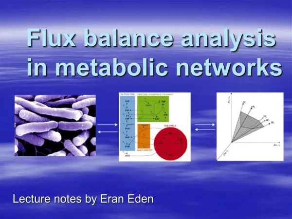
Stoichiometric analysis • Flux balance analysis (FBA) is a widely used stoichiometric analysis technique. • For a given growth condition (e.g. known input nutrients): • Assume that metabolic system operates in a steady state. • Assume certain constraints on system (mass-balance, flux limitations). • Assume an “objective” that is expected to be maximised by evolution (e.g. biomass production). • FBA can be used to predict reaction fluxes and essential enzymes under a given growth condition.
FBA example anoxic(no oxygen) hypoxic (limited oxygen) aerobic (unlimited oxygen) Pathways of starch storage at different phases of development in barley seeds Grafahrend-Belau Eet al. (2008)
Metabolic control analysis • Given kinetic parameters, we can calculate sensitivity of the flux through a given pathway to the inhibition of any enzyme involved. • This replaces the concept of a “rate-limiting step” in a pathway with the idea of control being shared to some degree between all enzymes, represented by each enzyme’s flux control coefficient, C. • Requires detailed kinetic model: currently limited to a few very well characterised pathways in specific organisms. C=1 0<C<1 C=0 Bakker BMet al. (2000)