Download
1 / 30
300 likes | 465 Views
Metabolic scaling relations in marine ecosystems trophic networks. Luca Palmeri Yuri Artioli Environmental System Analysis Lab Department of Chemical Processes Engineering UNIVERSITA’ DI PADOVA ITALY. Quo vadis ecosystem ?. or where are you going ecosystem ?

E N D
Metabolic scaling relations in marine ecosystems trophic networks Luca Palmeri Yuri Artioli Environmental System Analysis Lab Department of Chemical Processes Engineering UNIVERSITA’ DI PADOVA ITALY L. Palmeri
Quo vadis ecosystem ? or where are you going ecosystem ? Bendoricchio and Palmeri, 2005 Ecological Modelling184: 5–17 L. Palmeri
Each indicator gives a different point of view on systems’ state. Goal Functions are specific (or sectorial), not “global”. Indicators and Goal Functions S (IInd TD law) Maximum entropy equilibrium W(Lotka)Maximum power energy dissipation p (Prigogine) Minimal entropy production linear regime Em (Odum) Maximum empower energy quality (solar) Ex (Jørgensen) Maximum Exergy distance from equilibrium AMI, NC e Asc (Ulanowicz)Propensity to maximal Ascendency network organization Emx (Bastianoni & Marchettini) Minimum Em/Ex cost/benefit L. Palmeri
Total flow (TST) J13 1 3 J31 J21 2 J32 Ecosystem description (Ecological State) • Ecological Ecosystem Network analysis (flows and storages) • State a measurable property System analysis Holistic indicators from general system properties (e.g. allometries) Jikflow originated in i and entering k L. Palmeri
Trophic networks L. Palmeri
Ecosystem optimization Ecosystems try to optimize the flows and biomass Optimal networks show a balance between flows and biomass (lets say between costs and benefits) L. Palmeri
Network optimization • COST: supply the energy • Increase the quality of energy (higher trophic levels) • Foster energy transport (network articulation) • BENEFIT: respond to energy demand • catabolism • anabolism • development • OPTIMIZATION of • Stored energy (Biomass) • Supply/demand of resources (metabolites, energy flowing in the network) L. Palmeri
A General Metabolic Growth Model (von Bertalanffy) anabolism = metabolism - catabolism L. Palmeri
Weight vs. metabolism L. Palmeri
Weight vs. growth L. Palmeri
Allometric Metabolic Scaling • Biomass (B) • Flow out, metabolism (F) • Theorem: Banavar et al. (2002) for an optimal, balanced and direct D-dimensional network L. Palmeri
Supply-demand balance • Cost/BenefitOptimization Supply and Demand scale isometrically Supply rate Demand rate L. Palmeri
Allometric Metabolic Scaling • can be rewritten as • For an optimal network in D dimensions, the Theorem by Banavar et al. (2002) states L. Palmeri
If D = 3 If s1 = 0 from the theorem • If s1 = 0, supply rate independent of Biomass, ´= 2/3 • Ifs1 s2 , less energy is supplied than required, 2/3< ´<3/4 • Optimal condition: s1 = s2 , ´= 3/4 • Ifs1 s2 , more energy is supplied than required, ´> 3/4 Supply-demand balance L. Palmeri
as an Indicator of Trophic Network State • For biological systems D=3 Generally: 2/3 For a system, with B-independent supply: = 2/3 undersupplied: < 3/4 in optimal condition: = 3/4 oversupplied: > 3/4 L. Palmeri
Quo vadis ecosystem ? One answer might be: • Unfortunately ecosystems are not always represented by direct networks • they usually show feedbacks and matter recycling • A network with ¾ scaling could not correspond to an optimum and stable state • In that case the system could not employ overhead supply to compensate vulnerabilities to external pressures L. Palmeri
Quo vadis ecosystem ? According to the theoretical framework developed here, high a values (greater than 0.75 or close to 1) indicate the subsistence of one or several of the following network characteristics: • high supply/demand ratio • highly undirected network • flows redundancies • enhanced recycling • greater system resilience to external perturbations • high costs of maintainance for the network L. Palmeri
Quo vadis ecosystem ? Coversely, low a values (say equal to or less than 2/3) may indicate conditions spanning from ill-defined food web representation to undersupplied networks L. Palmeri
From the black book ofChristensen and Pauly (1993) SDB indicator, calculated for 13 trophic networks: a values in the range 0.29 - 2.50 L. Palmeri
N Lagoon of VeniceSDB Indicator L. Palmeri
N Lagoon of VeniceSDB Indicator L. Palmeri
N Lagoon of VeniceSDB Indicator L. Palmeri
N Lagoon of VeniceSDB Indicator L. Palmeri
N Lagoon of Venice SDB Indicator (annual) Fusina Sacca sessola Palude della Rosa Petta di Bo’ Ca’ Roman L. Palmeri
Lagoon of Venice SDB Indicator SDB is SENSITIVE accounting for very little differences in the same type of shallow water ecosystems, in different seasons (Fusina is different !) L. Palmeri
Lagoon of Venice SDB Indicator • SDB reflects DYNAMICS • isable to follow the seasonal succession, i.e. all the networks (except Fusina !) present a similar pattern of variation, i.e.: • Oversupplied in January (pp dormant, … ready to burst) • Balanced during spring (G&D are at a maximum level) • Undersupplied in late summer (decaying season) L. Palmeri
Lagoon of Venice SDB Indicator N Conclusions • Relatively easy to apply to “arbitrarily large” real networks, without • increasing computational demands • increasing the number of free parameters Allometric principles provide limit intervals (thresholds) for the indicator values and very general convergence schemes • Generality, applicable to very different systems • Sensitivity, distinguishes similar systems L. Palmeri
references • Almaas, E., B. Kovàcs, et al. (2004). “Global organization of metabolic fluxes in the bacterium Escherichia coli.” Nature427: 839-843. • Banavar, J. R., F. Colaiori, et al. (2001). “Scaling, Optimality, and Landscape Evolution.” Journal of Statistical Physics104(1/2). • Banavar, J. R., J. Damuth, et al. (2002). “Supply–demand balance and metabolic scaling.” Proceedings of the National Academy of Sciences99(16). • Banavar, J. R., A. Maritan, et al. (1999). “Size and form in efficient transportation networks.” Nature399: 130-132. • Bendoricchio, G. and Palmeri, L. (2005) “Quo vadis ecosystem?” Ecological Modelling 184: 5–17. • Garlaschelli, D., G. Caldarelli, et al. (2003). “Universal scaling relations in food webs.” Nature423: 165-168. • Niklas, K. J. and B. J. Enquist (2001). “Invariant scaling relationships for interspecific plant biomass productrion rates and body size.” Proceedings of the National Academy of Sciences98(5): 2922-2927. • West, G. B., J. H. Brown, et al. (2001). “A general model for ontogenic growth.” Nature413: 628-631. L. Palmeri