Download
1 / 17
170 likes | 314 Views
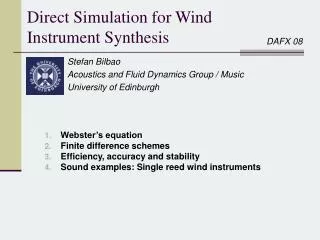
Direct Simulation for Wind Instrument Synthesis. DAFX 08. Stefan Bilbao Acoustics and Fluid Dynamics Group / Music University of Edinburgh. Webster’s equation Finite difference schemes Efficiency, accuracy and stability Sound examples: Single reed wind instruments. Webster’s Equation.

E N D
Direct Simulation for Wind Instrument Synthesis DAFX 08 Stefan Bilbao Acoustics and Fluid Dynamics Group / Music University of Edinburgh • Webster’s equation • Finite difference schemes • Efficiency, accuracy and stability • Sound examples: Single reed wind instruments
Webster’s Equation • Usual starting point for wind instrument models (and speech): an acoustic tube, surface area S(x) : S(x) x 0 L • Under various assumptions, velocity potential Y(x,t)satisfies: • Y(x,t)related to pressure p(x,t) and volume velocity u(x,t) by:
Single Reed Model • A standard one-mass reed model: . Bore uin . ur um -H pin pm 0 y x 0 • A driven oscillator: Linear oscillator terms Collision term Driving term Mouthpiece pressure drop Flow conservation Bore coupling Flow nonlinearity Flow induced by reed
Radiation Boundary Condition • At the radiating end (x=L), an approximate boundary condition is often given in impedance form: • Models inertial mass and loss. • BUT: not positive real not passive. • A better approximation (p.r., passive): • When converted to the time domain:
Finite Difference Scheme S • Sample bore profile at locations x = lh, l = 0,…,N • h = grid spacing h S1 SN S0 S2 SN-1 0 1 2 N-1 N Y • Introduce grid function Y, at locations x = lh, l = 0,…,N t = nk, n = 0,… • k = time step n+1 k … n n-1 0 1 2 N-1 N • Here is one particular finite difference scheme (explicit, 2nd order accurate) • Courant number l defined asl=ck/h
Can show (energy methods) that scheme is stable, over interior, when Stability and Special Forms • When l = 1, scheme simplifies to: …equivalent to Kelly-Lochbaum scattering method • When l = 1, and S = const., scheme simplifies further: …equivalent to digital waveguide (exact integrator)
Stability Condition and Tuning • Stability condition requires • For simplicity, would like to choose an h which divides L evenly, i.e., • Not possible for waveguide/Kelly-Lochbaum methods --- h=ck. Result: detuning, remedied using fractional delays. • In an FD scheme, can choose h as one wishes. Result: very minor dispersion/loss of audio bandwidth. Numerical cutoff: • Worst case near fs = 44.1 kHz, typical wind instrument dimensions:
Accuracy—Modal Frequencies • Numerical dispersion---normally a problem for FD schemes! • This is a 2nd order scheme---might expect severe mode detunings… • Not so… E.g., for a lossless clarinet bore… …calculated modal frequencies are nearly exact, over the entire spectrum
Accuracy—Transfer Impedance • Even under more realistic conditions (i.e., with radiation loss), behaviour is extremely good: • Transfer impedance (mouth radiating end): Red: exact (calculated at 400 kHz) Green: calculated at 44.1 kHz • Upshot: FD approximation converges very rapidly… • …“perceptually” exact, even at audio sample rate. • No compelling reason to look for better schemes…
Explicit Updating • Discretization of oscillator: Parameterized implicit discretization Implicit discretization Exact integrator possible for linear part of oscillator… Explicit update… Mouthpiece pressure drop Flow conservation Bore coupling Flow nonlinearity Flow induced by reed • Implicit discretization excellent stability properties • Unknowns always appear linearly…
Explicit Updating • Can find a flow path in order to update all the state variables (sequentially) Virtual grid point Excitation Reed state Bore Radiating end point • Similar to setting of “reflection-free port resistances” in linear WDF networks… • …but more general.
Note on Stability • The scheme for the bore + bell termination, in isolation, is guaranteed stable. • Situation more complicated when reed mechanism is connected. • Consider system under transient conditions (input pm = 0): True… Total energy Stored energy in bore Stored energy at bell Stored energy of reed Initial stored energy • System is dissipative state bounded for any initial conditions. • Under forced conditions, would like: Unfortunately this is false… Total energy Initial stored energy Energy supplied externally • Upshot: impossible to bound solutions of model system under forced conditions • Best one can do: ensure energy balance is respected in FD scheme…
Computational Cost For a given sample rate fs, bore length L, and wave speed c, the computational requirements are: • 2Lfs/c units memory • 4Lfs 2/c 6Lfs 2/c flops/sec. …independent of bore profile. Reed/tonehole/bell calculations are O(1) extra ops/memory per time step Example: clarinet 15 Mflops/sec., at fs = 44.1 kHz Not a lot by today’s standards…far faster than real time.
Toneholes • Not difficult to add in tonehole models: x 0 x(1) x(2) x(3) 1 • Can add terms pointwise to Webster’s equation: State of tonehole q Physical parameters defining tonehole q • In FD implementation, can be added anywhere along bore (Lagrange interpolation):
Sound Examples • Clarinet: • Saxophone: • Multiphonics/squeaks:
Conclusion • Disadvantages: • Costs more to compute than a typical waveguide model (but still not much!) • Advantages: • Bore modeling becomes trivial… • More general extensions possible (NL wave propagation) • Far more design freedom that, e.g., WG/WD methods