FisheRies
FisheRies. What I use R for. Current work: GAMMS with bayesian spikeslabGAM estimator to improve egg larvae biomass estimates Geostatistics Precision estimates of survey data Analyse acoustic data (abundance and biomass estimates) Previously: Create an online platform with catch anaysis.

FisheRies
E N D
Presentation Transcript
What I use R for • Current work: • GAMMS with bayesian spikeslabGAM estimator to improve egg larvae biomass estimates • Geostatistics • Precision estimates of survey data • Analyse acoustic data (abundance and biomass estimates) • Previously: • Create an online platform with catch anaysis
What is rApache • rApache project for web application development with R statistical language (http://rapache.net, developped by Jeroen Ooms, University of Utrecht) • Apache module named mod_R that embeds the R interpreter inside the web server, bundled with libapreq (Apache module for manipulating client request data) → transform R into a server-side scripting environment. • R package brew: templating framework for report generation, and it's perfect for generating HTML on the fly (syntax is similar to PHP, Ruby's erb module, Java Server Pages, and Python's psp module)
rApache and the fisherman • Combining statistics with fisherman's knowledge • Build a web application with • live data analysis of catch data • Look at correlations between environmental information and catches • Maps of environment and catches • Get the latest market prices • Get an insight into the value in the tank • Social media • Safety updates • Combining statistics with fisherman's knowledge • Build a web application with live data analysis of catch data • Look at correlations between environmental information and catches • Maps of environment and catches • Get an insight into the value in the tank • Social media • Safety updates
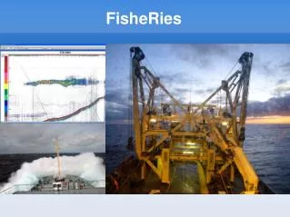
How does it work? Data collection Data processing • Temperature & Salinity profile • Currents • Sediments • Waves and Wind • Experience • Catch Information • Logbook & GPS 1) Data collection onboard from sensors 2) Auxiliary online data colleciton 3) Logbook entry into Excel form 4) Automated data upload 5) .rhtml pages – html and R anlayse and produce graphs Data Presentaion
Using rApache R code HTML form <% setContentType("text/html") %> <html> <body> <%require(ggplot2) library(ggplot2) data<-read.csv(".../data.csv") … i<-1%> <form method="post"> <select name="Trip"> <option value="all">Recorded Trips</option> <%for (i in 1:l){ …. }%> <input type="submit" value="PLOT"/> </form> <% a<-as.numeric(POST$Trip) trip<-(levels(factor(data$Trip.number))[a])%> <pre> <h2>Trip number: <%=trip%></h2> ... </body> </html> • Install rApache on any Linux/Unix or Mac Apache server • Define script folder for .R and .rhtml files • Create .rhtml files • → Normal HTML with R code embedded in <% … %> or call R script • Upload data or get data from forms • Create a user interface (for example with javascript libraries such as ExtJS)
googleVis • googleVis is an R package providing an interface between R and the Google Visualisation API • html code that contains the data and references to JavaScript functions hosted by Google http://code.google.com/p/google-motion-charts-with-r/ <% setContentType("text/html") myname <- ifelse(is.null(GET$name),'World',GET$name) %> <html> <head> <title>Catch information</title> </head> <body> <%library(ggplot2) library(googleVis) library(Hmisc) catch_3<-read.csv("/opt/local/apache2/htdocs/orion_data/catchwsed.csv") catch_3$Date<-as.Date(catch_3$Date)-(10*365+0.25*10)%> <%=gvisMotionChart(catch_3, idvar="Species", timevar="Haul", options=list(width=500, height=450))$html$chart%> </body></html> </html>
Second part • Combine mackerel acoustic and egg data • Use the DIDSON acoustic camera to automatically detect fish
R for a fisheries scientist • Stock assessments • 2 main types of surveys I currently work with: • Egg/larvae surveys e.g. Triennial Horse mackerel/Mackerel egg survey • Acoustic surveys e.g. Acoustic herring survey, Acoustic blue whiting survey
From egg countings to SSB • Stock information based on triennial egg survey • Mackerel hard to detect acoustically as they do not have a swimbladder • Duration Stage 1: Ln(hours)=-1.61*ln(Temp.)+7.76 Temperature at 5m ð Ds_hours= e^Ln(hours) • Egg abundance per m2: Ae=Ce*S*D/V Ce=Counted eggs S=raising factor D=sampling depth V=filtered Volume • Daily egg production: DEP=24*Ae / DS hours Area ICES square: cos(lat)*30*1853.2*30*1853.2 • Total annual egg production: TAEP=DEP*72* Area • Spawning stock biomass SSB=SR*TAEP/TF SR=Sex ratio=1:1=2, Total fecundity=1401eggs/g/female
Mackerel egg production curve 2002 using qplot from ggplot2 qplot(data=d.eggs.plot,Julian.Days,Daily.egg.production)+geom_line(colour="red",size=2) #Create lineplot with qplot ggsave(file=paste("output/EggProductionCurve",year,".png",sep="")) #Save file as png Counted eggs per m2 for the 3 survey periods in 2002 using qplot from ggplot2 survey.area<-as.data.frame(map("world", xlim=c(-2,10), ylim=c(52,62),plot=FALSE)[c("x","y")]) #create map using package maps area<-qplot(x,y,data=survey.area,geom="path") # include map in qplot q<-area + geom_text(aes(x=Lon, y=Lat, label=round(DEPR,1),colour=DEPR),size=2.5,data=data_mbl) #add values of DEPR & colour them q<-q + scale_x_continuous("Longitude",breaks=floor(min(data_mbl$Lon)):ceiling(max(data_mbl$Lon))) # define scales for X axis q<-q+scale_y_continuous("Latitude",breaks=floor(min(data_mbl$Lat)):ceiling(max(data_mbl$Lat))) # define scales for Y axis q<-q + opts(legend.position = "none") # remove legend q<-q+ opts(title = paste("Daily egg production Part",i,year,sep=" "),size=13) # Add title q
Mackerel in the North Sea Calculations relatively easy but do not provide any error estimates Improvement: model data using GAMs or GAMMs with bayesion factor estimator and combine with acoustic data ####SpikeSlabGam library(spikeSlabGAM) ... f1<-log(eggs.m2+1) ~ Lon+Lat+Temp.5m f2<-log(eggs.m2+1) ~ (Lon+Lat+Temp.5m + B.Depth)^2 f3<-log(eggs.m2+1) ~ (Lon+Lat+Temp.5m + B.Depth)^3 fa<-log(eggs.m2+1)~(S.depth+Vol.filt+J.Day)^2+(sm(Lon)+sm(Lat)+sm(Temp.5m))^2 mcmc<-list(nChains=8,chainlength=1000,burnin=500,thin=5) m1<-spikeSlabGAM(formula=f1, family="gaussian", data=ddd, mcmc=mcmc) m2<-spikeSlabGAM(formula=f2, family="gaussian", data=ddd, mcmc=mcmc) m3<-spikeSlabGAM(formula=f3, family="gaussian", data=ddd, mcmc=mcmc) ma<-spikeSlabGAM(formula=fa, family="gaussian", data=ddd, mcmc=mcmc) Packages used: GAMM: spikeSlabGAM Time: fields Visualisation: ggplot (integrated in spikeSlabGAM) ####GAM library(mgcv) ... mac.t5.bd<-gam(log(Egg.m2+1)~s(Lon,Lat,k = 10)+s(Temp.5m)+ s(B.depth), data = data05.in) mac.t5<-gam(log(Egg.m2+1)~s(Lon,Lat,k = 10)+s(Temp.5m), data = data05.in) Packages used: GAM: mgcv Time: fields Visualisation: maps
Egg abundance map GAM 2002 #Define the area lon<-seq(minlon,maxlon,1/2) lat<-seq(minlat,maxlat,1/2) llo<-length(lon) lla<-length(lat) zz<-array(NA,llo*lla) Lat<-0 Lon<-0 a<-1 for (i in 1:lla) { for (j in 1:llo) { Lat[a]<-lat[i] Lon[a]<-lon[j] a<-a+1 j<-j+1 } i<-i+1 } ###VISULISATION A data$log.net.area <- 0*data$Lon # make offset column zz[data$ind]<-(predict(mac.t5,abcd)) #predict the values png(paste("map.GAM_t5_",fn,"_",year,".png",sep="")) #write to file image(lon,lat,matrix(zz,llo,lla),col=topo.colors(100), cex.lab=1,cex.axis=1,xlim=c(-4,10),ylim=c(50,60)) contour(lon,lat,matrix(zz,llo,lla),add=TRUE) map('world', fill = F, col = 1:10,xlim=c(-4,10),ylim=c(50,60),add=T) #Add world map contours dev.off()
Egg abundance maps using spikeslabGAM and ggplot2 for 2002 • Simply plot(modelname,labels=c(“var1:var2")) • Using ggplot2 within the spikeSlabGAM with labels defining the selected variables plot(m2,labels=“Temp.5m") respectively Lon, Lat plot(m2,labels=c(“Lon:Lat"))
DIDSON Acoustic camera • Acoustic lens, 96 beams, 0.3° opening, Frequency 1.8 MHz • Currently used to count & measure length of fishes • Can it be used to look at the acoustic blind zone? • Stability?
Target strength measurements Copper Tungsten Carbide qplot(copper$TS_uncomp, geom = "density",ylab="Density", xlab="TS uncompensated") qplot(copper$Ping_number,copper$TS_uncomp,ylab="uncompensated TS (dB)",xlab="Ping number")