Download
1 / 35
350 likes | 920 Views
MODULE 5. Unsteady State Heat Conduction . UNSTEADY HEAT TRANSFER.

E N D
MODULE 5 Unsteady State Heat Conduction
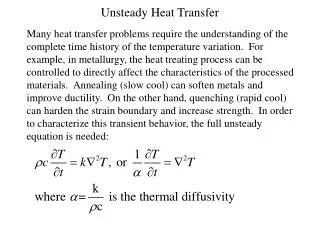
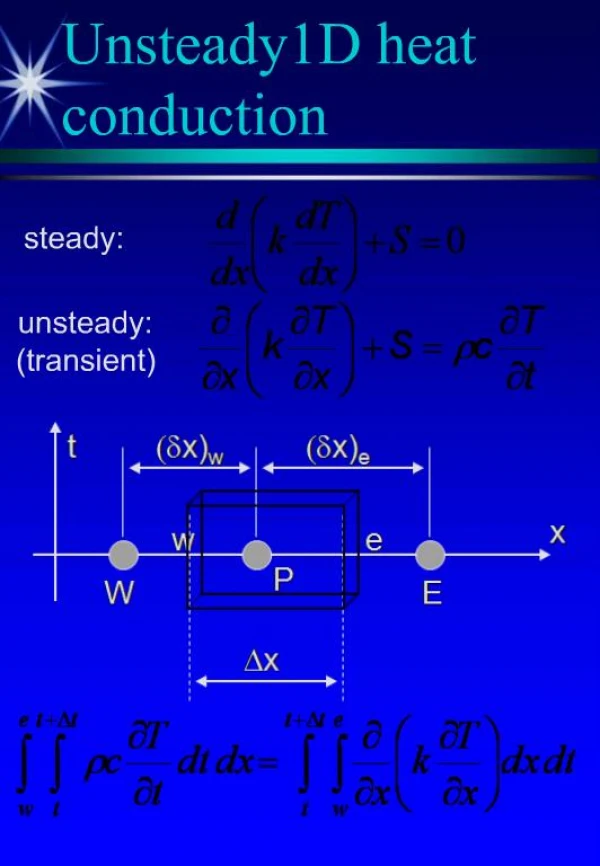
UNSTEADY HEAT TRANSFER Many heat transfer problems require the understanding of the complete time history of the temperature variation. For example, in metallurgy, the heat treating process can be controlled to directly affect the characteristics of the processed materials. Annealing (slow cool) can soften metals and improve ductility. On the other hand, quenching (rapid cool) can harden the strain boundary and increase strength. In order to characterize this transient behavior, the full unsteady equation is needed:
“A heated/cooled body at Ti is suddenly exposed to fluid at T with a known heat transfer coefficient . Either evaluate the temperature at a given time, or find time for a given temperature.” Q: “How good an approximation would it be to say the bar is more or less isothermal?” A: “Depends on the relative importance of the thermal conductivity in the thermal circuit compared to the convective heat transfer coefficient”.
Biot No. Bi • Defined to describe the relative resistance in a thermal circuit of the convection compared Lc is a characteristic length of the body Bi→0: No conduction resistance at all. The body is isothermal. Small Bi: Conduction resistance is less important. The body may still be approximated as isothermal (purple temp. plot in figure) Lumped capacitance analysis can be performed. Large Bi: Conduction resistance is significant. The body cannot be treated as isothermal (blue temp. plot in figure).
Solid Total Resistance= Rexternal + Rinternal GE: BC: Solution: Transient heat transfer with no internal resistance: Lumped Parameter Analysis Valid for Bi<0.1
Note: Temperature function only of time and not of space! Lumped Parameter Analysis • - To determine the temperature at a given time, or • To determine the time required for the • temperature to reach a specified value.
Thermal diffusivity:(m² s-1) Lumped Parameter Analysis
Lumped Parameter Analysis Define Fo as the Fourier number (dimensionless time) and Biot number The temperature variation can be expressed as T = exp(-Bi*Fo)
Spatial Effects and the Role of Analytical Solutions The Plane Wall: Solution to the Heat Equation for a Plane Wall with Symmetrical Convection Conditions
The Plane Wall: • Note: Once spatial variability of temperature is included, there is existence of seven different independent variables. • How may the functional dependence be simplified? • The answer is Non-dimensionalisation. We firstneed to understand the physics behind the phenomenon, identify parameters governing the process, and group them into meaningful non-dimensional numbers.
Dimensionless temperature difference: Dimensionless coordinate: Dimensionless time: The Biot Number: The solution for temperature will now be a function of the other non-dimensional quantities Exact Solution: The roots (eigenvalues) of the equation can be obtained from tables given in standard textbooks.
and time ( ): The One-Term Approximation Variation of mid-plane temperature with time From tables given in standard textbooks, one can obtain and as a function of Bi. Variation of temperature with location Change in thermal energy storage with time:
Graphical Representation of the One-Term Approximation: The Heisler Charts Midplane Temperature:
Temperature Distribution Change in Thermal Energy Storage • Assumptions in using Heisler charts: • Constant Ti and thermal properties over the body • Constant boundary fluid T by step change • Simple geometry: slab, cylinder or sphere
Radial Systems Long Rods or Spheres Heated or Cooled by Convection Similar Heisler charts are available for radial systems in standard text books. Important tips: Pay attention to the length scale used in those charts, and calculate your Biot number accordingly.
Unsteady Heat Transfer in Semi-infinite Solids • Solidification process of the coating layer during a thermal spray operation is an unsteady heat transfer problem. As we discuss earlier, thermal spray process deposits thin layer of coating materials on surface for protection and thermal resistant purposes, as shown. The heated, molten materials will attach to the substrate and cool down rapidly. The cooling process is important to prevent the accumulation of residual thermal stresses in the coating layer.
liquid Coating with density r, latent heat of fusion: hsf d S(t) solid Substrate, k, a Unsteady Heat Transfer in Semi-infinite Solids(contd…)
Example • As described in the previous slide, the cooling process can now be modeled as heat loss through a semi-infinite solid. (Since the substrate is significantly thicker than the coating layer) The molten material is at the fusion temperature Tf and the substrate is maintained at a constant temperature Ti. Derive an expression for the total time that is required to solidify the coating layer of thickness d.
Example • Assume the molten layer stays at a constant temperature Tf throughout the process. The heat loss to the substrate is solely supplied by the release of the latent heat of fusion. Heat transfer from the molten material to the substrate (q=q”A)
Example (contd...) • Identify that the previous situation corresponds to the case of a semi-infinite transient heat transfer problem with a constant surface temperature boundary condition. This boundary condition can be modeled as a special case of convection boundary condition case by setting h=, therefore, Ts=T).
Example (contd...) • Use the following values to calculate: k=120 W/m.K, a=410-5 m2/s, r=3970 kg/m3, and hsf=3.577 106 J/kg, Tf=2318 K, Ti=300K, and d=2 mm
Example (contd…) • d(t) t1/2 • Therefore, the layer solidifies very fast initially and then slows down as shown in the figure • Note: we neglect contact resistance between the coating and the substrate and assume temperature of the coating material stays the same even after it solidifies. • To solidify 2 mm thickness, it takes 0.43 seconds.
Example (contd…) • What will be the substrate temperature as it varies in time? The temperature distribution is:
x 0 . 79 = = - = - T ( x 0 . 01 , t ) 2318 2018 erf 79 . 06 2318 2018 erf t t Example (contd…) • For a fixed distance away from the surface, we can examine the variation of the temperature as a function of time. Example, 1 cm deep into the substrate the temperature should behave as:
Example (contd...) • At x=1 cm, the temperature rises almost instantaneously at a very fast rate. A short time later, the rate of temp. increase slows down significantly since the energy has to distribute to a very large mass. • At deeper depth (x=2 & 3 cm), the temperature will not respond to the surface condition until much later.
= = - = - T ( x , t 1 ) 2318 2018 erf 79 . 06 2318 2018 erf 79 . 06 x x t Example (contd...) • We can also examine the spatial temperature distribution at any given time, say at t=1 second. • Heat penetrates into the substrate as shown for different time instants. • It takes more than 5 seconds for the energy to transfer to a depth of 5 cm into the substrate • The slopes of the temperature profiles indicate the amount of conduction heat transfer at that instant.
Numerical Methods for Unsteady Heat Transfer • Unsteady heat transfer equation, no generation, constant k, two-dimensional in Cartesian coordinate: • We have learned how to discretize the Laplacian operator into system of finite difference equations using nodal network. For the unsteady problem, the temperature variation with time needs to be discretized too. To be consistent with the notation from the book, we choose to analyze the time variation in small time increment Dt, such that the real time t=pDt. The time differentiation can be approximated as:
m,n+1 m-1,n m+1, n m,n m,n-1 Finite Difference Equations • From the nodal network to the left, the heat equation can be written in finite difference form:
Nodal Equations • Some common nodal configurations are listed in table for your reference. On the third column of the table, there is a stability criterion for each nodal configuration. This criterion has to be satisfied for the finite difference solution to be stable. Otherwise, the solution may be diverging and never reach the final solution.
Nodal Equations (contd…) • For example, Fo1/4. That is, aDt/(Dx)2 1/4 and Dt(1/4a)(Dx)2. Therefore, the time increment has to be small enough in order to maintain stability of the solution. • This criterion can also be interpreted as that we should require the coefficient for TPm,n in the finite difference equation be greater than or equal to zero. • Question: Why this can be a problem? Can we just make time increment as small as possible to avoid it?
Finite Difference Solution • Question: How do we solve the finite difference equation derived? • First, by specifying initial conditions for all points inside the nodal network. That is to specify values for all temperature at time level p=0. • Important: check stability criterion for each points. • From the explicit equation, we can determine all temperature at the next time level p+1=0+1=1. The following transient response can then be determined by marching out in time p+2, p+3, and so on.
x 1 3 2 Example • Example: A flat plate at an initial temperature of 100 deg. is suddenly immersed into a cold temperature bath of 0 deg. Use the unsteady finite difference equation to determine the transient response of the temperature of the plate. L(thickness)=0.02 m, k=10 W/m.K, a=1010-6 m2/s, h=1000 W/m2.K, Ti=100C, T=0C, Dx=0.01 m Bi=(hDx)/k=1, Fo=(aDt)/(Dx)2=0.1 There are three nodal points: 1 interior and two exterior points: For node 2, it satisfies the case 1 configuration in table.


![Chapter 3: Unsteady State [ Transient ] Heat Conduction](https://cdn1.slideserve.com/2468294/chapter-3-unsteady-state-transient-heat-conduction-dt.jpg)