Download
1 / 43
430 likes | 517 Views
Variance reduction and Brownian Simulation Methods. Yossi Shamai Raz Kupferman The Hebrew University. . Dumbbell models. All (incompressible) fluids are governed by mass-momentum conservation equations. u ( x,t ) = velocity ( x,t ) = polymeric stress. q. Dumbbell models.

E N D
Variance reduction and Brownian Simulation Methods Yossi Shamai Raz Kupferman The Hebrew University
Dumbbell models All (incompressible) fluids are governed by mass-momentum conservation equations u(x,t)= velocity (x,t) = polymericstress
q Dumbbell models The polymers are modeled by two beads connected by a spring (dumbbell) . The conformation is modeled by an end-to-end vector q. less affect more affect (q,x,t) = pdf.
q The (random) conformations are distributed according to a density function (q,x,t), which satisfies an evolution equation advection deformation diffusion The stress is an ensemble average of polymeric conformations, g(q) = qF(q)
Conservation laws (macroscopic dynamics) The stress Polymeric density distribution (microscopic dynamics) • Problem: high dimensionality • Assumption: 1-D
Example (Semi-linear systems): if g(q) = q2, andb(q,u) = b(u) q then (x,t)satisfies the PDE • Closable systems can be solved by standard methods. • Brownian simulations can be used for non-closable systems. Closable systems In certain cases, a PDE for (x,t) can be derived, yielding a closed-form system for u(x,t),(x,t).
Outline 1. Brownian simulation methods 2. Some mathematical preliminaries on spatial correlations 3. A variance reduction mechanism in Brownian simulations 4. Examples
Brownian simulations The average stress (x,t) is an expectation with respect to a stochastic process q(x,t) with PDF (q,x,t) PDE SPDE q(x,t) is simulated by a collection of realizationsqi(x,t). The stress is approximated by an empirical mean
L2-valuedBrownian motion B(x,t) is a random function of time and space. For fixed x, B(x,t) is a real-valued Brownian motion. Finite norm A reminder: real-valued Brownian motion B(t) is a random function of time. Almost surely continues. Independent increments. B(t)-B(s) ~ N(0,t-s).
Symmetry: c(x,y) = c(y,x). c(x,x) = 1. L2 - function: Spatial correlations B(x,t) is characterized by the spatial correlation function
Uniform Oscillatory Discretization Piecewise constant uncorrelated Spatial correlations (cont.) An L2 - function is a correlation function iff a. c(x,x) = 1. b. It has a “square root” in L2
Spatial correlations (cont.) • No spatially uncorrelated L2-valued Brownian motion. • Spatially uncorrelated noise has meaning only in a discrete setting. It is a sequence of piecewise constant standard Brownian motions, uncorrelated at any two distinct steps, that converges to 0.
For any f,g in L2 Spatial correlations (cont.) Spatial correlations can be alternatively described by Correlation operators • C is nonnegative, symmetric and trace class. • No Id-correlated Brownian motion (trace Id = ∞ ).
SPDEs (Stochastic Partial Differential Equations) Ito’s integral • F,G are operators SDEs versus SPDEs SDEs (Stochastic Differential Equations) Ito’s integral
SPDEs PDE (Fokker-Plank) SPDE SDEs versus SPDEs SDEs PDE (Fokker-Plank) SDE • q(x,t) has spatial correlation.
• Consistency: for every x, q(x,0) ~ (q,x,0). Lemma: Let(u,,q)be a solution for the stochastic system on some time interval[0,T]. Let(q,x,t)be the PDF corresponding to q(x,t). Then(u,,)is a solution for the deterministic system on[0,T]. Brownian simulationsunifying approach • Equivalence class insensitive to spatial correlations.
• Advantages: • No Fokker-plank equation. • Easy to simulate. Disadvantages: 1. No error analysis. 2. Variance is O(n-1). Brownian simulation methods The stochastic process q is simulated by n “realizations” driven by i.i.d Brownian motions. Expectation is approximated by an empirical mean with respect to the realizations:
Brownian simulation methods The approximation The system Correlation affects approximation but not the exact solution CONNFFESSIT (Calculations of Non Newtonian Fluids Finite Elements and Stochastic Simulation Techniques) - Piecewise constant uncorrelated noise (Ottinger et al. 1993) BCF - Spatially uniform noise (Hulsen et al. 1997) Error reduction ?
Goals The error of the Brownian simulations is Prove that e(n,t)0. Reduce the error by choosing the spatial correlation ofthe Brownian noise: Step 1. Express e(n,t)as a function F(c). Step 2. Minimize F(c). The idea of adapting correlation to minimize variance first proposed by Jourdain et al. (2004) in the context of shear flow with a specific FEM scheme.
The Brownian simulation is Example An “integral-type” system
The Brownian simulation at t=20 (dotted curve) The (normalized) error as a function of time “smooth” simulation Large error (1.47) Results: n = 2000 with spatially uniform noise ( c(x,y) = 1 ). Brownian simulation Brownian simulation The stress Stress
The (normalized) error as a function of time reduced error (1.06) Results: n = 2000 with piecewise constant uncorrelated noise. The Brownian simulation at t=20 (dotted curve) “noisy” simulations
Error analysis We want to analyze the error of the Brownian simulations Lets demonstrate the analysis for semi-linear system…
Example (Semi-linear systems): if g(q) = q2, andb(q,u) = b(u) q then (x,t)satisfies the PDE • Closable systems can be solved by standard methods. • Brownian simulations can be used for non-closable systems. Closable systems In certain cases, a PDE for (x,t) can be derived, yielding a closed-form system for u(x,t),(x,t).
An analogous evolution equation for T(x,t) is derived Error analysis for Semi-linear systems We want to estimate the error of the Brownian simulations In semi-linear systems, the stress field (x,t)satisfies a PDE • Linearize (properly)
The function F can be also expressed in terms of the correlation operator C, Theorem 1. To leading order: where and k is a kernel function determined by the parameters.
Error analysis for Closable systems Theorem1. To leading order in n, • F is convex • In principle, the analysis is the same • Proof is restricted to closable systems
Find a sequence of correlations cnS such that F(cn)converge to The optimization problem Minimize F(c) over the domain: S = {c(x,y) : c has a root in L2, c(x,x) = 1} • In general, there is no minimizer Difficulties: A. Infinite dimensional optimization problem. B. S is not compact.
Theorem 2. The sequence of errors converges (as k∞ ) to the optimal error Finite dimensional approximations 1. Set a natural k. 2. Discretize the problem to a k-point mesh
The F-D optimization problem • We want to minimize F(ck) over Sk. • ck(x,y)is indexed by k2 mesh points(xi ,xj) (matrix). • SymmetricPositive-Semi-Definite. • ck(xi ,xi)= 1. The F-D optimization problem is: Minimize F(A), A is k-by-k symmetric PSD Subject to Aii = 1, i=1,…,k F is convex SDP algorithms (Semi-Definite Programming)
So what did we do? • Developed a unifying approach for a variance reduction mechanism in Brownian simulations. • Formulated an optimization problem (in infinite dimensions). • Showed that it is amenable to a standard algorithm (SDP).
In stochastic formulation, The Brownian simulation is Example 1 A linear advection-dissipation equation in [0,1].
The error is Variance independent of correlations (no reduction) Insights: the dynamics (advection and dissipation) do not mix different points in space. Thus, the error only ‘sees’ diagonal elements of the correlations, which are fixed by the constraints.
Example 2 An “integral-type” system (x[0,1]): Closable:
The Brownian simulation at t=20 (dotted curve) The (normalized) error as a function of time “smooth” simulation Large error (1.47) Results: n = 2000 with spatially uniform noise ( c(x,y) = 1 ). (BCF) Brownian simulation Brownian simulation The stress Stress
The (normalized) error as a function of time optimal error (1.06) Results: n = 2000 with piecewise constant uncorrelated noise (CONNFFESSIT). The Brownian simulation at t=20 (dotted curve) “noisy” simulations
The error is • g(x,y,t) is singular on the diagonal (x=y), and a smooth positive function off the diagonal. • c(x,x) = 1 Why?… the optimal error is obtained by taking c 0 (CONNFESSIT).
The system: Closable: set Example 3: 1-D planar Shear flow model. (Jourdain et al. 2004)
Any sequence ck 0yields the optimal error (e.g, spatially constant uncorrelated) To leading order, the error of the Brownian simulations is • C - the spatial correlation operator. • K(t) - a nonnegative bounded operator.
So is CONFFESSIT always optimal? • No! • We can construct a problem for • which e(n,t) = n-1(const + Tr[K(t)C]) • for K(t) bounded and not PSD. • Theorem. If the semi-groups are Hilbert-Schmidt (they have L2-kernels) then CONNFFESSIT is optimal.
Some further thoughts… • The spatial correlation of the initial data q(x,0) may also be considered. • Non-closable systems? • Gain insights about the optimal correlation by understand relations between type of equation and optimal correlation.