Download
1 / 147
1.52k likes | 2.13k Views
Assumptions of multiple regression. Assumption of normality Transformations Assumption of linearity Assumption of homoscedasticity Script for testing assumptions Practice problems. Assumptions of Normality, Linearity, and Homoscedasticity.

E N D
Assumptions of multiple regression Assumption of normality Transformations Assumption of linearity Assumption of homoscedasticity Script for testing assumptions Practice problems
Assumptions of Normality, Linearity, and Homoscedasticity • Multiple regression assumes that the variables in the analysis satisfy the assumptions of normality, linearity, and homoscedasticity. (There is also an assumption of independence of errors but that cannot be evaluated until the regression is run.) • There are two general strategies for checking conformity to assumptions: pre-analysis and post-analysis. In pre-analysis, the variables are checked prior to running the regression. In post-analysis, the assumptions are evaluated by looking at the pattern of residuals (errors or variability) that the regression was unable to predict accurately. • The text recommends pre-analysis, the strategy we will follow.
Assumption of Normality • The assumption of normality prescribes that the distribution of cases fit the pattern of a normal curve. • It is evaluated for all metric variables included in the analysis, independent variables well as the dependent variable. • With multivariate statistics, the assumption is that the combination of variables follows a multivariate normal distribution. • Since there is not a direct test for multivariate normality, we generally test each variable individually and assume that they are multivariate normal if they are individually normal, though this is not necessarily the case.
Assumption of Normality:Evaluating Normality There are both graphical and statistical methods for evaluating normality. • Graphical methods include the histogram and normality plot. • Statistical methods include diagnostic hypothesis tests for normality, and a rule of thumb that says a variable is reasonably close to normal if its skewness and kurtosis have values between –1.0 and +1.0. • None of the methods is absolutely definitive. • We will use the criteria that the skewness and kurtosis of the distribution both fall between -1.0 and +1.0.
Assumption of Normality:Histograms and Normality Plots On the left side of the slide is the histogram and normality plot for a occupational prestige that could reasonably be characterized as normal. Time using email, on the right, is not normally distributed.
Assumption of Normality:Hypothesis test of normality The hypothesis test for normality tests the null hypothesis that the variable is normal, i.e. the actual distribution of the variable fits the pattern we would expect if it is normal. If we fail to reject the null hypothesis, we conclude that the distribution is normal. The distribution for both of the variable depicted on the previous slide are associated with low significance values that lead to rejecting the null hypothesis and concluding that neither occupational prestige nor time using email is normally distributed.
Assumption of Normality:Skewness, kurtosis, and normality Using the rule of thumb that a rule of thumb that says a variable is reasonably close to normal if its skewness and kurtosis have values between –1.0 and +1.0, we would decide that occupational prestige is normally distributed and time using email is not. We will use this rule of thumb for normality in our strategy for solving problems.
Assumption of Normality:Transformations • When a variable is not normally distributed, we can create a transformed variable and test it for normality. If the transformed variable is normally distributed, we can substitute it in our analysis. • Three common transformations are: the logarithmic transformation, the square root transformation, and the inverse transformation. • All of these change the measuring scale on the horizontal axis of a histogram to produce a transformed variable that is mathematically equivalent to the original variable.
Assumption of Normality:When transformations do not work • When none of the transformations induces normality in a variable, including that variable in the analysis will reduce our effectiveness at identifying statistical relationships, i.e. we lose power. • We do have the option of changing the way the information in the variable is represented, e.g. substitute several dichotomous variables for a single metric variable.
Assumption of Normality:Computing “Explore” descriptive statistics To compute the statistics needed for evaluating the normality of a variable, select the Explore… command from the Descriptive Statistics menu.
Assumption of Normality:Adding the variable to be evaluated Second, click on right arrow button to move the highlighted variable to the Dependent List. First, click on the variable to be included in the analysis to highlight it.
Assumption of Normality:Selecting statistics to be computed To select the statistics for the output, click on the Statistics… command button.
Assumption of Normality:Including descriptive statistics First, click on the Descriptives checkbox to select it. Clear the other checkboxes. Second, click on the Continue button to complete the request for statistics.
Assumption of Normality:Selecting charts for the output To select the diagnostic charts for the output, click on the Plots… command button.
Assumption of Normality:Including diagnostic plots and statistics First, click on the None option button on the Boxplots panel since boxplots are not as helpful as other charts in assessing normality. Finally, click on the Continue button to complete the request. Second, click on the Normality plots with tests checkbox to include normality plots and the hypothesis tests for normality. Third, click on the Histogram checkbox to include a histogram in the output. You may want to examine the stem-and-leaf plot as well, though I find it less useful.
Assumption of Normality:Completing the specifications for the analysis Click on the OK button to complete the specifications for the analysis and request SPSS to produce the output.
Assumption of Normality:The histogram An initial impression of the normality of the distribution can be gained by examining the histogram. In this example, the histogram shows a substantial violation of normality caused by a extremely large value in the distribution.
Assumption of Normality:The normality plot The problem with the normality of this variable’s distribution is reinforced by the normality plot. If the variable were normally distributed, the red dots would fit the green line very closely. In this case, the red points in the upper right of the chart indicate the severe skewing caused by the extremely large data values.
Assumption of Normality:The test of normality Since the sample size is larger than 50, we use the Kolmogorov-Smirnov test. If the sample size were 50 or less, we would use the Shapiro-Wilk statistic instead. The null hypothesis for the test of normality states that the actual distribution of the variable is equal to the expected distribution, i.e., the variable is normally distributed. Since the probability associated with the test of normality is < 0.001 is less than or equal to the level of significance (0.01), we reject the null hypothesis and conclude that total hours spent on the Internet is not normally distributed. (Note: we report the probability as <0.001 instead of .000 to be clear that the probability is not really zero.)
Transformations:Transforming variables to satisfy assumptions • When a metric variable fails to satisfy the assumption of normality, homogeneity of variance, or linearity, we may be able to correct the deficiency by using a transformation. • We will consider three transformations for normality, homogeneity of variance, and linearity: • the logarithmic transformation • the square root transformation, and • the inverse transformation • plus a fourth that may be useful for problems of linearity: • the square transformation
Transformations:Computing transformations in SPSS • In SPSS, transformations are obtained by computing a new variable. SPSS functions are available for the logarithmic (LG10) and square root (SQRT) transformations. The inverse transformation uses a formula which divides one by the original value for each case. • For each of these calculations, there may be data values which are not mathematically permissible. For example, the log of zero is not defined mathematically, division by zero is not permitted, and the square root of a negative number results in an “imaginary” value. We will usually adjust the values passed to the function to make certain that these illegal operations do not occur.
Transformations:Two forms for computing transformations • There are two forms for each of the transformations to induce normality, depending on whether the distribution is skewed negatively to the left or skewed positively to the right. • Both forms use the same SPSS functions and formula to calculate the transformations. • The two forms differ in the value or argument passed to the functions and formula. The argument to the functions is an adjustment to the original value of the variable to make certain that all of the calculations are mathematically correct.
Transformations:Functions and formulas for transformations • Symbolically, if we let x stand for the argument passes to the function or formula, the calculations for the transformations are: • Logarithmic transformation: compute log = LG10(x) • Square root transformation: compute sqrt = SQRT(x) • Inverse transformation: compute inv = 1 / (x) • Square transformation: compute s2 = x * x • For all transformations, the argument must be greater than zero to guarantee that the calculations are mathematically legitimate.
Transformations:Transformation of positively skewed variables • For positively skewed variables, the argument is an adjustment to the original value based on the minimum value for the variable. • If the minimum value for a variable is zero, the adjustment requires that we add one to each value, e.g. x + 1. • If the minimum value for a variable is a negative number (e.g., –6), the adjustment requires that we add the absolute value of the minimum value (e.g. 6) plus one (e.g. x + 6 + 1, which equals x +7).
Transformations:Example of positively skewed variable • Suppose our dataset contains the number of books read (books) for 5 subjects: 1, 3, 0, 5, and 2, and the distribution is positively skewed. • The minimum value for the variable books is 0. The adjustment for each case is books + 1. • The transformations would be calculated as follows: • Compute logBooks = LG10(books + 1) • Compute sqrBooks = SQRT(books + 1) • Compute invBooks = 1 / (books + 1)
Transformations:Transformation of negatively skewed variables • If the distribution of a variable is negatively skewed, the adjustment of the values reverses, or reflects, the distribution so that it becomes positively skewed. The transformations are then computed on the values in the positively skewed distribution. • Reflection is computed by subtracting all of the values for a variable from one plus the absolute value of maximum value for the variable. This results in a positively skewed distribution with all values larger than zero. • When an analysis uses a transformation involving reflection, we must remember that this will reverse the direction of all of the relationships in which the variable is involved. Out interpretation of relationships must be adjusted accordingly.
Transformations:Example of negatively skewed variable • Suppose our dataset contains the number of books read (books) for 5 subjects: 1, 3, 0, 5, and 2, and the distribution is negatively skewed. • The maximum value for the variable books is 5. The adjustment for each case is 6 - books. • The transformations would be calculated as follows: • Compute logBooks = LG10(6 - books) • Compute sqrBooks = SQRT(6 - books) • Compute invBooks = 1 / (6 - books)
Transformations:The Square Transformation for Linearity • The square transformation is computed by multiplying the value for the variable by itself. • It does not matter whether the distribution is positively or negatively skewed. • It does matter if the variable has negative values, since we would not be able to distinguish their squares from the square of a comparable positive value (e.g. the square of -4 is equal to the square of +4). If the variable has negative values, we add the absolute value of the minimum value to each score before squaring it.
Transformations:Example of the square transformation • Suppose our dataset contains change scores (chg) for 5 subjects that indicate the difference between test scores at the end of a semester and test scores at mid-term: -10, 0, 10, 20, and 30. • The minimum score is -10. The absolute value of the minimum score is 10. • The transformation would be calculated as follows: • Compute squarChg = (chg + 10) * (chg + 10)
Transformations:Transformations for normality Both the histogram and the normality plot for Total Time Spent on the Internet (netime) indicate that the variable is not normally distributed.
Transformations:Determine whether reflection is required Skewness, in the table of Descriptive Statistics, indicates whether or not reflection (reversing the values) is required in the transformation. If Skewness is positive, as it is in this problem, reflection is not required. If Skewness is negative, reflection is required.
Transformations:Compute the adjustment to the argument In this problem, the minimum value is 0, so 1 will be added to each value in the formula, i.e. the argument to the SPSS functions and formula for the inverse will be: netime + 1.
Transformations:Computing the logarithmic transformation To compute the transformation, select the Compute… command from the Transform menu.
Transformations:Specifying the transform variable name and function First, in the Target Variable text box, type a name for the log transformation variable, e.g. “lgnetime“. Third, click on the up arrow button to move the highlighted function to the Numeric Expression text box. Second, scroll down the list of functions to find LG10, which calculates logarithmic values use a base of 10. (The logarithmic values are the power to which 10 is raised to produce the original number.)
Transformations:Adding the variable name to the function Second, click on the right arrow button. SPSS will replace the highlighted text in the function (?) with the name of the variable. First, scroll down the list of variables to locate the variable we want to transform. Click on its name so that it is highlighted.
Transformations:Adding the constant to the function Following the rules stated for determining the constant that needs to be included in the function either to prevent mathematical errors, or to do reflection, we include the constant in the function argument. In this case, we add 1 to the netime variable. Click on the OK button to complete the compute request.
Transformations:The transformed variable The transformed variable which we requested SPSS compute is shown in the data editor in a column to the right of the other variables in the dataset.
Transformations:Computing the square root transformation To compute the transformation, select the Compute… command from the Transform menu.
Transformations:Specifying the transform variable name and function First, in the Target Variable text box, type a name for the square root transformation variable, e.g. “sqnetime“. Third, click on the up arrow button to move the highlighted function to the Numeric Expression text box. Second, scroll down the list of functions to find SQRT, which calculates the square root of a variable.
Transformations:Adding the variable name to the function Second, click on the right arrow button. SPSS will replace the highlighted text in the function (?) with the name of the variable. First, scroll down the list of variables to locate the variable we want to transform. Click on its name so that it is highlighted.
Transformations:Adding the constant to the function Following the rules stated for determining the constant that needs to be included in the function either to prevent mathematical errors, or to do reflection, we include the constant in the function argument. In this case, we add 1 to the netime variable. Click on the OK button to complete the compute request.
Transformations:The transformed variable The transformed variable which we requested SPSS compute is shown in the data editor in a column to the right of the other variables in the dataset.
Transformations:Computing the inverse transformation To compute the transformation, select the Compute… command from the Transform menu.
Transformations:Specifying the transform variable name and formula First, in the Target Variable text box, type a name for the inverse transformation variable, e.g. “innetime“. Second, there is not a function for computing the inverse, so we type the formula directly into the Numeric Expression text box. Third, click on the OK button to complete the compute request.
Transformations:The transformed variable The transformed variable which we requested SPSS compute is shown in the data editor in a column to the right of the other variables in the dataset.
Transformations:Adjustment to the argument for the square transformation It is mathematically correct to square a value of zero, so the adjustment to the argument for the square transformation is different. What we need to avoid are negative numbers, since the square of a negative number produces the same value as the square of a positive number. In this problem, the minimum value is 0, no adjustment is needed for computing the square. If the minimum was a number less than zero, we would add the absolute value of the minimum (dropping the sign) as an adjustment to the variable.
Transformations:Computing the square transformation To compute the transformation, select the Compute… command from the Transform menu.
Transformations:Specifying the transform variable name and formula First, in the Target Variable text box, type a name for the inverse transformation variable, e.g. “s2netime“. Second, there is not a function for computing the square, so we type the formula directly into the Numeric Expression text box. Third, click on the OK button to complete the compute request.
Transformations:The transformed variable The transformed variable which we requested SPSS compute is shown in the data editor in a column to the right of the other variables in the dataset.
Assumption of Normality:The test of normality Using the rule of thumb for evaluating normality with the skewness and kurtosis statistics, we look at the table of descriptive statistics. The skewness and kurtosis for the variable both exceed the rule of thumb criteria of 1.0. The variable is not normally distributed.