Download
1 / 60
610 likes | 970 Views
Signals & systems Ch.3 Fourier Transform of Signals and LTI System. Signals and systems in the Frequency domain. Fourier transform. Time [sec]. Frequency [sec -1 , Hz]. 3.1 Introduction. Orthogonal vector => orthonomal vector What is meaning of magnitude of H?.

E N D
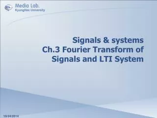
Signals & systemsCh.3 Fourier Transform of Signals and LTI System
Signals and systems in the Frequency domain Fourier transform Time [sec] Frequency [sec-1, Hz] KyungHee University
3.1 Introduction • Orthogonal vector => orthonomal vector • What is meaning of magnitude of H? Any vector in the 2- dimensional space can be represented by weighted sum of 2 orthonomal vectors Fourier Transform(FT) Inverse FT KyungHee University
3.1 Introduction cont’ • CDMA? Orthogonal? Any vector in the 4- dimensional space can be represented by weighted sum of 4 orthonomal vectors Orthonormal function? KyungHee University
3.2 Complex Sinusoids and Frequency Response of LTI Systems cf) impulse response How about for complex z? (3.1) How about for complex s? (3.3) Magnitude to kill or not? Phase delay KyungHee University
Fourier transform Time domain frequency domain discrete time Continuous time z-transform Laplace transform (periodic) - (discrete) (discrete) - (periodic) KyungHee University
3.6 DTFT: Discrete-Time Fourier Transform (discrete) (periodic) (a-periodic) (continuous) (3.31) (3.32) KyungHee University
3.6 DTFT Example 3.17 Example 3.17 DTFT of an Exponential Sequence Find the DTFT of the sequence Solution : = 0.5 = 0.9 x[n] = nu[n]. magnitude = 0.5 = 0.9 phase KyungHee University
3.6 DTFT Example 3.18 Example 3.18 DTFT of a Rectangular Pulse Let Find the DTFT of Solution : (square) (sinc) Figure 3.30 Example 3.18. (a) Rectangular pulse in the time domain. (b) DTFT in the frequency domain. KyungHee University
3.6 DTFT Example 3.18 KyungHee University
3.6 DTFT Example 3.19 Example 3.19 Inverse DTFT of a Rectangular Spectrum Find the inverse DTFT of Solution : (sinc) (square) Figure 3.31 (a) Rectangular pulse in the frequency domain. (b) Inverse DTFT in the time domain. KyungHee University
3.6 DTFT Example 3.20-21 Example 3.20 DTFT of the Unit Impulse Find the DTFT of Solution : (impulse) - (DC) Example 3.21 Find the inverse DTFT of a Unit Impulse Spectrum. Solution : (impulse train) (impulse train) KyungHee University
3.6 DTFT Example 3.23 Example 3.23 Multipath Channel : Frequency Response Solution : (a) a = 0.5ej2/3. (b) a = 0.9ej2/3. (a) a = 0.5ej2/3. (b) a = 0.9ej2/3. KyungHee University
3.7 CTFT (continuous aperiodic) (continuous aperiodic) CTFT (3.26) Inverse CTFT (3.35) Condition for existence of Fourier transform: KyungHee University
3.7 CTFT Example 3.24 Example 3.24 FT of a Real Decaying Exponential Find the FT of Solution : Therefore, FT not exists. LPF or HPF? Cut-off from 3dB point? KyungHee University
3.7 CTFT Example 3.25 Example 3.25 FT of a Rectangular Pulse Find the FT of x(t). Solution : (square) (sinc) Example 3.25. (a) Rectangular pulse. (b) FT. KyungHee University
3.7 CTFT Example 3.25 Example 3.26 Inverse FT of an Ideal Low Pass Filter!! Fine the inverse FT of the rectangular spectrum depicted in Fig.3.42(a) and given by Solution : (sinc) -- (square) KyungHee University
3.7 CTFT Example 3.27-28 Example 3.27 FT of the Unit Impulse Solution : (impulse) - (DC) Example 3.28 Inverse FT of an Impulse Spectrum Find the inverse FT of Solution : (DC) (impulse) KyungHee University
3.7 CTFT Example 3.29 Example 3.29 Digital Communication Signals Rectangular (wideband) Separation between KBS and SBS. Narrow band Figure 3.44 Pulse shapes used in BPSK communications. (a) Rectangular pulse. (b) Raised cosine pulse. KyungHee University
3.7 CTFT Example 3.29 Solution : Figure 3.45 BPSK (a) rectangular pulse shapes (b) raised-cosine pulse shapes. the same power constraints KyungHee University
3.7 CTFT Example 3.29 rectangular pulse. One sinc Raised cosine pulse 3 sinc’s The narrower main lobe, the narrower bandwidth. But, the more error rate as shown in the time domain Figure 3.47 sum of three frequency-shifted sinc functions. KyungHee University
Fourier transform Time domain frequency domain Discrete time Continuous time KyungHee University
3.9.1 Linearity Property KyungHee University
3.9.1 Symmetry Properties • Real and Imaginary Signals (real x(t)=x*(t)) (conjugate symmetric) (3.37) (3.38) KyungHee University
3.9.2 Symmetry Properties of FT • EVEN/ODD SIGNALS (even) (real) (odd) (pure imaginary) For even x(t), real KyungHee University
3.10 Convolution Property (convolution) (multiplication) But given change the order of integration KyungHee University
3.10 Convolution Property Example 3.31 Example 3.31 Convolution problem in the frequency domain Input to a system with impulse response Find the output Solution: KyungHee University
3.10 Convolution Property Example 3.32 Example 3.32 Find inverse FT’S by the convolution property Use the convolution property to find x(t), where Ex 3.32 (p. 261). (a) Rectangular z(t). (b) KyungHee University
3.10.2 Filtering Continuous time Discrete time(periodic with 2π LPF HPF BPF Figure 3.53 (p. 263) Frequency dependent gain (power spectrum) kill or not (magnitude) KyungHee University
3.10 Convolution Property Example 3.34 Example 3.34 Identifying h(t) from x(t) and y(t) The output of an LTI system in response to an input is . Find frequency response and the impulse response of this system. Solution: But But note KyungHee University
3.10 Convolution Property Example 3.35 EXAMPLE 3.35 Equalization(inverse) of multipath channel or Consider again the problem addressed in Example 2.13. In this problem, a distorted received signal y[n] is expressed in terms of a transmitted signal x[n] as Then KyungHee University
3.11 Differentiation and Integration Properties EXAMPLE 3.37 The differentiation property implies that KyungHee University
3.11 Differentiation and Integration Properties • 예제한 두개 KyungHee University
3.11.2 DIFFERENTIATION IN FREQUENCY Differentiate w.r.t. ω, Then, Example 3.40 FT of a Gaussian pulse Use the differentiation-in-time and differentiation-in-frequency properties for the FT of the Gaussian pulse, defined by and depicted in Fig. 3.60. and Then (But, c=?) Figure 3.60 (p. 275) Gaussian pulse g(t). KyungHee University
Laplacetransform and z transform KyungHee University
3.11.3 Integration Ex) Prove Note where a=0 We know since linear Fig. a step fn. as the sum of a constant and a signum fn. KyungHee University
Differentiation and Integration Properties Common Differentiation and Integration Properties. KyungHee University
3.12.1 Time-Shift Property Fourier transform of time-shifted z(t) = x(t-t0) Note that x(t-t0) = x(t) * δ(-t0) and Table 3.7 Time-Shift Properties of Fourier Representations KyungHee University
3.12 Time-and Frequency-Shift Properties Example) Figure 3.62 KyungHee University
3.12.2 Frequency-Shift Property Recall Table 3.8 Frequency-Shift Properties KyungHee University
3.12.2 Frequency-Shift Property Example 3.42 FT by Using the Frequency-Shift Property Solution: We may express as the product of a complex sinusoid and a rectangular pulse KyungHee University
3.12 Shift Properties Ex. 3.43 Example 3.43 Using Multiple Properties to Find an FT Sol) Let and Then we may write By the convolution and differentiation properties The transform pair KyungHee University
3.12 Shift Properties Ex. 3.43 Example 3.43 Using Multiple Properties to Find an FT Sol) Let and Then we may write By the convolution and differentiation properties The transform pair s KyungHee University
3.13 Inverse FT: Partial-Fraction Expansions • 3.13.1 Inverse FT by using N roots, partial fraction KyungHee University
3.13 Inverse FT: Partial-Fraction Expansions • 3.13.1 Inverse FT by using Let then N roots, partial fraction KyungHee University
Inverse FT: Partial-Fraction Expansions KyungHee University
3.13.2 Inverse DTFT • 3.13.2 where Then KyungHee University
Inverse FT: Partial-Fraction Expansions KyungHee University
3.13.2 Inverse DTFT by z-transform • 3.13.2 where Then KyungHee University
3.13 Inverse FT Example 3.45 Example 3.45 Inversion by Partial-Fraction Expansion Solution: Using the method of residues described in Appendix B, We obtain And Hence, 2011.5.4 KyungHee University