Download
1 / 23
230 likes | 340 Views
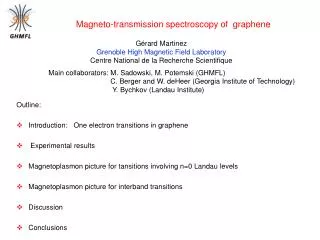
Magneto-transmission spectroscopy of graphene. Gérard Martinez Grenoble High Magnetic Field Laboratory Centre National de la Recherche Scientifique. Outline: Introduction: One electron transitions in graphene Experimental results

E N D
Magneto-transmission spectroscopy of graphene Gérard Martinez Grenoble High Magnetic Field Laboratory Centre National de la Recherche Scientifique Outline: • Introduction: One electron transitions in graphene • Experimental results • Magnetoplasmon picture for tansitions involving n=0 Landau levels • Magnetoplasmon picture for interband transitions • Discussion • Conclusions Main collaborators: M. Sadowski, M. Potemski (GHMFL) C. Berger and W. deHeer (Georgia Institute of Technology) Y. Bychkov (Landau Institute)
n = 3 n = 2 A n = 1 E10 n = 0 B C D n = -1 n = -2 n = -3 Introduction One electron transitions in graphene The band structure of graphene is composed of two cones located at two inequivalent corners K and K’ of the Brillouin zone at which conduction and valence band merge. For each valley: at B=0 For finite value of B Each LL 0 is four times degenerated due to spin and valley degeneracy. Depending on the filling factor, different optical transitions are allowed either of « cyclotron type » (A ) or of « interband transitions type » (C and D) or mixed (B) In experiments an effective value of the velocitycalled larger than vF is found for all transitions (Sadowski et al., PRL , 97, 266405 (2006)) Here we take the value of vF= 0.86 106 m/s
Experimental results :Graphene samples The SiC-4H sample is graphetized: heated to1500 °C in high vacuum sublimation of Si atoms leaving behind C planes. A variety of characterizations techniques lead to the conclusion that the active part of this type of structures consists of a few graphene layers. We got likely a structure with broken sheets as: One expects structured samples such as: The dc conductivty data show that the carrier concentration is in the range of 4 1012 cm-2 which is due to the built-in electric field at the interface SiC-graphene and self-consistent calculations indicate that it should reduced to zero within the next five layers.
FTS spectrometer Brucker IFS-66v Reference Sample Bolometer (Si) Experimental results : Instrumentation Magneto-transmission measurements are performed in an absolute way using a rotating sample holder working in situ in order to eliminate the magnetic dependent response of the detector. Sample: graphitized SiC Reference: pure SiC The SiC substrate with a thikness of about 300 m is opaque for energies between 85 and 200 meV.
n = 3 n = 2 A n = 1 E10 n = 0 B C D n = -1 n = -2 n = -3 Experimental results Example of transmission spectrum in graphene C B D A The relative intensity of transition A versus transition Bgives the electronic density of the layer which depending on the sample is of the order of 1010 cm-2. (Fermi energy less than 10 meV)
Transmission experiments: main features C Two kinds of transitions were followed constinuously for magnetic fields up to 4T A first estimate of their energy position demonstrate that they vary like B1/2, leading to assume that they reflect the presence of graphene layers in the sample. These transitions correspond to an oscillator strength which also clearly increases with the magnetic field like B1/2 in contrast to conventional 2DEG. B
Transmission experiments: global behavior All transitions vary linearly with the square root of the magnetic field with a slope, independent of the transitions corresponding to an effective velocity of: much larger than vF. All these findings lead to the conclusion that all observed transitions are originating from graphene layers doped at a level much lower than the one measured in transport measurements. Sadowski et al., PRL , 97, 266405 (2006)
Transmission experiments: exfoliated graphene Z. Jiang et al., cond-mat/0703822 Measurements at fixed field: ratio of transmission at nu= +/-2 with respect to nu= -10 Significantly larger than values found with SiC-G samples Ratio of effective velocities 1.05
N0+ 2 c N0+ 1 b a N0 Magnetoplasmon plasmon approach Magnetoplasmon excitations in conventional 2DEG Transitions among Landau levels are not single electron transitions + electron-electron interactions CR is an excitonic transition magneto-plasmon dispersion MP model developped for any filling factor Phys. Rev. B 66, 193312 (2002) also including the corresponding optical conductivity. Phys. Rev. B 72, 195328 (2005) Three one-electron transitions Three MP curves describing the dispersion of excitonic-like transitions
Magnetoplasmon picture in graphene In the magnetoplasmon picture, derived in the Hartree-Fock+RPA approximations, all the spin and valley dependent transitions could be a priori mixed: Call the creation operator governing the transition n’n, with spin , in a valley : Difference of exchange energies of the two levels n and n’ Electron-hole interaction Same spin, same valley Simultaneous creation and destruction of an exciton at different points of the Brillouin zone for any value of the spin and in any valley. The model assumes that the Coulomb energy Ec=e2/lB is smaller than the different energy transitions.
n = 1 B n = 0 E10 n = -1 Valley K Valley K’ Magnetoplasmon picture for transitions involving the n=0 Landau Levels Results of the model are presented for filling factors < 2 Because the interaction is mainly important for energy transitions which are of the same order of magnitude, it is possible to treat the problem independently for the different types of transitions: B, C and others For transitions B there are five possible transitions corresponding to the energy E10. Comparaison of the tansition energy E10 and Coulomb energy Ec= e2/lB : For graphene : E10(meV)= 31.1 (B(T))1/2 Ec(meV)= 11.2 (B(T))1/2 E1/Ec = 2.78 independent on the field For a 2DEG (GaAs) : c(meV)= 1.7 B(T) Ec (meV) = 4.45 (B(T))1/2 c/Ec = 0.38 (B(T))1/2 The condition Ec<E1 is better fulfilled for Graphene than for GaAs. One assumes that there is a splitting DS of the valleys K and K’ larger than the spin splitting in such a way the electrons remain in the same valley (here K) for any value of n<2.
Magnetoplasmon picture for transitions involving the n=0 Landau Levels One has to solve the Hamiltonian for the exciton energies: E10= 2.77 e2/lB Two degenerate solutions for non integer value of and three degenerate solutions for = 1 or 2. • Without introducing DV corrections, • all dispersion curves converge • to a single value for klB 0. • One single line (red curve) in infrared absorption Curves are displayed with respect to the one-electron energy E10. Only one dispersion curve (red curve) will give rise to singularities in the density of states which could possibly be seen in Raman experiments.
Magnetoplasmon picture for transitions involving the n=0 Landau Levels : transition B For k values of the exciton 0, the Hamiltonian is essentially diagonal with terms involving the difference of exchange contributons and .The MP energy is: Independent of the filling factor! With that formulation C1 diverges and the summation has to be truncated but will remain much larger than 3/4 a0. Therefore the evolution of the energy of the transition B with will display a slope larger than vF. On the other hand the intensity of the transition remains proportional to (vF)2!
n = 2 n = 1 I n = 0 J n = -1 n = -2 Valley K Valley K’ Magnetoplasmon picture for transitions C One has to treat now 8 transitions four corresponding to n=-1 n=2 (labelled I ) and four corresponding to n=-2 n=1 (labelled J ). In the one electron picture all these transitions correspond to the same energy : In Coulomb units E21= 6.693 The resulting matrix to be diagonalized has a very high degree of degeneragy.
Magnetoplasmon picture for transitions involving the LL n=-2,-1 to n= 1,2 (transition C) The one electron picture gives an energy E21= 6.693 e2 /klB Results are identical for =1 or 2 and very sligthly dependent on for non integer values Two single solutions (left part of the figure) and two groups of three times degenerate solutions . At klB 0 there are two dictinct solutions for integer values of n. The only optical active transitions are those corresponding to the non degenrate solutions
Magnetoplasmon picture for interband transitions at klB0 Transition C For k lB 0, the Hamiltonian is essentially diagonal and for integer values of n there is a splitting . ( very small) The mean variation of the transition is given by: Also divergent but : DC2 converges Therefore one can write: All the divergence remains in C1.
Magnetoplasmon picture for transitions involving the LL n=-3,-2 to n= 2,3 (transitionD) The one electron picture gives an energy E32= 8.722 e2 /klB Results are identical for =1 or 2 and very sligthly dependent on for non integer values Two single solutions (left part of the figure) and two groups of three degenerate solutions . At klB 0 there are two dictinct solutions for integer values of n. The only active optical transitions are those corresponding to the non degenrate solutions.
Magnetoplasmon picture for interband transitions at klB0 Transition D For k lB 0, the Hamiltonian is essentially diagonal and for integer values of n there is a splitting . ( very small) The mean variation of the transition is given by: Again divergent but : DC3 converges Therefore one can write: All the divergence remains in C1.
Magnetoplasmon picture for interband transitions at klB0 Model to treat the divergence of C1 The most reliable experimental results, because obtained on a large scale of magnetic field are those relative to the transitions C and D and E. For these transitions, the effective velocity is : We use this experimentall value to determine the upper index of LL, Nmax beyond which the summation for C1 is truncated. The scaling is performed with the transition C This requires the imput of a value for vF: Taking vF = 0.86 106 m/s Nmax= 28, C1 = 0.880 and C2 = -0.157 Taking vF = 0.88 106 m/s Nmax= 17, C1 = 0.805 and C2 = -0.158 for the transition D In both cases: for the transition E for the transition B The effective velocity of the transition B is found to be lower than that of the two next interband transitions by about 4%. Not observed in SiC-G
Electron-phonon interaction in Graphene Models with different types of electron-phonon interactions predict a splitting of the valley which is as big as the spin splitting and vary linearly with the magnetic field. J. Yan et al., March meeting Denver (2007) Fuchs and Lederer, PRL, 98, 016803 (2007) All the optical branches are expected to give a strong electron-phonon interaction which also renormalizes the Fermi velocity by decreasing it.
Consequences of the introduction of the electron-phonon interaction What is expected if we introcude a valley splitting DV ? Models with different types of electron-phonon interactions predict a splitting of the valley which is as big as the spin splitting and vary linearly with the magnetic field. Consequences: In such a case one expects a splitting of the transitionB which should provide a direct measurement of DV . Transitions C and the following ones should not be splitted but their variation with the field should acquire a component linear in the field. B B’ C C Splitting observed in transport measurements in high fields: Y.Zhang et al., PRL, 96,136806 (2006)
Conclusions of the magnetoplasmon model • There exist characteristic dispersion relations for graphene which depends on the optical transition. They are different for transitions implying the n=0 LL (B) and those related to interband transitions (C, D,E ..). The results are not depending on the existence of a splitting between valleys K and K’. • For the transitionB,near klB 0, one finds a single MP tansition in the absence of the valley spiltting DV which should be splited by DV . • For interband transitions, near klB 0, the MP transitions are splitted due to the exchange terms but no extra splitting is expected due to the introduction of DV. • The variation of the optical energies of the transitions, near klB 0, with the magnetic field corresponds to an effective velocity higher than the Fermi velocity vF. • This effective velocity is found to be lower for the transition Bthan for interband transitions by about 4%. • The oscillator strength of the transitions remains proportional to (vF)2.
Problems which remain to be solved • There are on the experimental side divergences between experimental results obtained on SiC-G and exfoliated Graphene. Why? • We do not have yet any direct measurement of the electron-phonon interaction in Graphene or of the splitting DV . • If the electron-electron interactions “open” the gap (increase of the renormalized Fermi velocity) the strong electron-phonon interaction in C-based compound, including Graphene will tend to decrease it. What is their relative weight?. In experiments we measure a combination of both and it is even not very clear on theoritical grounds that this combination should be the same with and without magnetic field !!