Download
1 / 76
760 likes | 885 Views
A Performance Comparison of Multi-Hop Wireless Ad Hoc Network Routing Protocols. Broch et al Presented by Brian Card. Outline. Introduction NS enhancements Protocols: DSDV TORA DRS AODV Evaluation Conclusions. Introduction. Node1. Node2. Node3. Node4. Introduction. Node1.

E N D
A Performance Comparison of Multi-Hop Wireless Ad Hoc Network Routing Protocols Broch et al Presented by Brian Card
Outline Introduction NS enhancements Protocols: DSDV TORA DRS AODV Evaluation Conclusions
Introduction Node1 Node2 Node3 Node4
Introduction Node1 Node2 Node3 Node4 How Does Node 1 Communicate with Node 4?
Introduction Node1 Node2 Node3 Node4 How Does Node 1 Communicate with Node 4?
What if the network looks like this? Node1 Node3 Node8 Node7 Node5 Node4 Node2 Node6
What if the network looks like this? Node1 Node3 Node8 Node7 Node5 Node4 Node2 Node6
What if the network looks like this? Node1 Node3 Node8 Node7 Node5 Node4 Node2 Node6 Multiple paths from Node 1 to Node 4, which one is the best?
What if the network is mobile? Node1 Node3 Node8 Node7 Node5 Node4 Node2 Node6
What if the network is mobile? • Need intelligent routing between nodes
Mobile Ah-Hoc Networks • Hop between nodes when point to point communication is not possible • Nodes can leave and join the network at any time • Link characteristics between nodes unpredictable • Nodes may move! • In and out of range • Can cause variations in link characteristics
Protocols for Ad-Hoc Mobile Networks • Need to quickly and accurately find routes to different nodes • Need to be able to recalculate based on changing node positions or changes in link characteristics • Need to be efficient
Issues with Protocols for Ad-Hoc Mobile Networks • Several protocols already exist, how do we know which one to choose? • No performance evaluation comparing protocols • Simulation tools don’t accurately model mobile networks • No support for physical layer characteristics • No support for MAC layer • No support for node positions • This paper attempts to address these issues
Outline Introduction NS enhancements Protocols: DSDV TORA DRS AODV Evaluation Conclusions
NS Enhancements • NS (Network Simulator) is a discrete event simulator widely used for network performance evaluation • Extensive support for simulating TCP • No support for Wi-Fi MAC layer or physical layer • No position information
Physical Layer Additions to NS • 1/r2 attenuation model within reference distance (100m), 1/r4 attenuation model afterwards • Movement is modeled using position as a function of time using flat surface or topographical map • Power is tracked for each interface, when model predicts power is lower than receive threshold the packet is marked as dropped in error • Carrier sensing threshold is used to treat low power transmissions as noise • Propagation delay is also accounted for
MAC Layer additions to NS • Physical lay feed packets to MAC Layer • virtual carrier sensing is used at the MAC layer (RTS/CTS) • ACK packets are transmitted for unicast packets, retransmits occur from sender until ACKs are received
Other NS Updates • ARP (Address Resolution Protocol) is used for determining link-layer IP addresses • This is important because ARP REQUEST is broadcast and can interact with protocols • Each node has a 50 packet send queue. Drop-tail is used for queue management
Outline Introduction NS enhancements Protocols: DSDV TORA DRS AODV Evaluation Conclusions
Protocols • Authors implemented 4 different routing protocols • Some changes were made to the protocols to improve performance • The following changes were made to all of them: • Broadcasts and broadcast responses were jittered using a random delay between 0 and 10 ms to prevent synchronization • Routing packets were transmitted before data or ARP packets • This was to ensure that routing information propagated quickly • Link breakage was detected at the MAC layer except for DSDV
DSDV: Destination-Sequenced Distance Vector • Hop by hop distance vector routing protocol • Each node keeps a routing table with three fields for each destination: • Next hop • Sequence number • Metric • Routers are chosen based on sequence number and metric • Higher sequence number (newer route) wins first • Afterwards lower metric wins
DSDV: Destination-Sequenced Distance Vector • Nodes are periodically sending out sequence numbers which represent the ‘freshness’ of a link • When a link is broken, the nodes marks the metric as infinite • This causes routes to avoid that node • When the node comes back up, a new sequence number is generated and packets flow over the new link
DSDV Implementation • MAC protocol link breakages are not used • Authors noted when using MAC level breakages if a single link is broken the node becomes unreachable • Sequence number from the breakage becomes higher than other sequence numbers and becomes the preferred route • This causes the node to be completely unreachable (packet drops) until it can advertise and create a new sequence number
DSDV and DSDV-SQ • Original protocol description is ambiguous about when to send updates • Authors use an additional scheme they call DSDV-SQ (SQ for sequence number) which also sends out updates when a sequence number changes • This increases overhead, but provides better performance since broken links are detected sooner • Authors use this for all experiments and provide a comparison to DSDV at the end of the paper
TORA: Temporarily-Ordered Routing Algorithm • Routes are discovered on-demand • Network is modeled like a system of pipes with the packets being water in the pipes • Protocol is layered on top of IMEP to provide guaranteed in-order packet delivery • Other protocols do not require this • IMEP can be used for address resolution but the authors did not use this and used ARP for all protocols • IMEP also groups TORA and IMEP control messages into blocks called ‘object blocks’
TORA Basic Usage • QUERY packet broadcasted when a packet needs to be delivered to some address. • Packet moves through the network until it reaches the destination or a node that can route to the destination • When a QUERY packet is received an UPDATE packet is then sent with the node’s height with respect to that destination • Height is used to calculate the flow parameters • Greater height indicates more resistance • Each node that receives an UPDATE packet then adjusts it’s own height for that destination to be larger than the value in the UPDATE packet • When a link is broken, the height it updated to a local maximum and an UPDATE packet is sent out
Implementation • TORA sensitive to intervals used for IMEP ‘object blocks’, no guidance given by specification with respect to these parameters • authors chose 150-250ms • TORA nodes must have an accurate picture of the network • In order guaranteed delivery very important • If A can’t reach B then B must also think that it can’t reach A
DSR: Dynamic Source Routing • Each packed contains the entire route needed to deliver the packet • Each node does not maintain up to date routing information • No route advertisements that are used in other protocols
DSR Basic Usage • When a packet needs to be sent a ROUTE REQUEST is broadcasted • Either the destination node or another node that knows how to get to the destination respond with a ROUTE REPLY • Nodes cache messages and use them to aggressively limit the spread of ROUTE REQUEST messages • This process is called Route Discovery • When network topology changes, a ROUTE ERROR is used to indicate a broken link • Used to invalidate caches • This process is called Route Maintenance
DSR Implementation • Only support bi-directional links • ROUTE REPLY packets traverse same links the ROUTE REQUESTS were sent over • The first time a ROUTE REQUEST is made, send it to only the neighbor nodes • This reduces network usage and allows a sender to query the caches of it’s neighbors and optimize for the use case where the destination is in range • If nothing comes back, re-broadcast and allow propagation. • All nodes scan for ROUTE ERRORs in promiscuous mode • Also if a node hears a packet and it can route to the destination, it sends a pre-emptive ROUTE REPLY • Finally, routers will change the route if it knows the next hop is not available and it has another path in it’s cache
AODV: Ad Hoc On-Demand Distance Vector • Combination of DSR and DSDV • Combines Route Discovery and Route Maintenance from DSR • With hop-by-hop routing, sequence numbers and beacons from DSDV • Creates both forward and reverse routes from nodes when ROUTE REQUESTs are sent out • Nodes only remember the next hop and not the entire route • Periodic HELLO messages are broadcasted by nodes, if a node misses 3 HELLOs from a neighbor the node is marked down, and this state is broadcasted
AODV Implementation • Authors created variation called AODV-LL which uses the link layer to detect broken links • Removes overhead from periodic HELLO messages, but broken links can only be detected on demand! • AODV-LL performs slightly better than AODV • Changed ROUTE REPLY timeout from 120 seconds to 6 seconds • Protocol reacts to dropped packets much faster with this lower timeout
Outline Introduction NS enhancements Protocols: DSDV TORA DRS AODV Evaluation Conclusions
Experimental Setup • Major component of the paper is to test how protocols react with moving nodes and physical layer / MAC simulations • 50 nodes for a 900 second simulation • Rectangular area to test longer routes • Generate 210 different scenarios, run each algorithm against each scenario and compare results
Experimental Scenarios • Each scenario was a pre-recorded sequence of events • Nodes switched between being stationary and moving, stationary time was called pause time • 7 different pause times: 0, 30, 60, 120, 600, 900 • 0 means constantly moving, 900 is no movement • 10 randomly generated movement patterns for each pause time • 20 meters/sec max speed, 10 meter/sec avg speed
Data Sources • Varied the number of sources from 10, 20, 30 • Packet sizes of 64 bytes or 1024 bytes • 4 packets per second • All sources use UDP traffic transmitted at constant bit rates • 3 sets of sources X 70 movement patterns = 210 scenarios • No TCP sources
Measured Shorted Path Lengths • Simulation software measures the number of hops for each path for each scenario • Changing speed has little effect on number of hops • 2.6 hops on average
Measured Shorted Path Lengths • Simulation software measures the number of hops for each path for each scenario • Changing speed has little effect on number of hops • 2.6 hops on average Number of hops for 20 m/s vs 1 m/s is about the same
Link Connectivity Changes • Number of times that a node goes in or out of range of another node
Routing Overhead • “Total number of packets transmitted during the simulation. For packets sent over multiple hops, each transmission of the packet (each hop) counts as one transmission”
Routing Overhead DSDV-SQ is constant DSR has lowest overhead
Packet Delivery Ratio • ratio between number of packets originated by the application layer CBR sources and the number of packets received at the destination. Higher is better.
Packet Delivery Ratio – Varying the Number of Sources • Figure 4 shows several charts, each chart has a protocol responds to 10, 20 and 30 CBR sources based on pause time. • Higher values are better