Solving Einstein's field equations
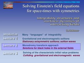
Solving Einstein's field equations. for space-times with symmetries. Integrability structures and. nonlinear dynamics of. interacting fields. G.Alekseev. Many “languages” of integrability. Introduction. Gravitational and electromagnetic solitons

Solving Einstein's field equations
E N D
Presentation Transcript
Solving Einstein's field equations for space-times with symmetries Integrability structures and nonlinear dynamics of interacting fields G.Alekseev Many “languages” of integrability Introduction Gravitational and electromagnetic solitons Stationary axisymmetric solitons; soliton waves Lecture 1 Monodromy transform approach Solutions for black holes in the external fields Lecture 2 Solving of the characteristic initial value problems Colliding gravitational and electromagnetic waves Lecture 3
Monodromy tarnsform approach to solution of integrable reductions of Einstein’s field equations. Lecture 2 Monodromy data as coordinates in the space of solutions Direct and inverse problems of the monodromy transform. Integral equation form of the field equations and infinite hierarchies of their solutions Some applications: solutions for black holes in external gravitational and electromagnetic fields
Integrable reductions of the Einstein's field equations Gravitational fields in vacuum: Elektrovacuum Einstein - Maxwell fields: Gravity model with axion, dilaton and E-H fields Bosonic sector of heterotic string effective action:
Reduced dynamical equations – generalized Ernst eqs. -- Vacuum -- Electrovacuum -- Einstein- Maxwell- Weyl
Generalized (matrix) Ernst equations for D4 gravity model with axion, dilaton and one gauge field: 1) Generalized (dxd-matrix) Ernst equations for heterotic string gravity model in D dimensions: 1) 1) A.Kumar and K.Ray (1995); D.Gal’tsov (1995), O.Kechkin, A. Herrera-Aguilar, (1998),;
Monodromy Transform approach to solving of Einstein's equations Free space of the mono- dromy data functions: The space of local solutions: (Constraint: field equations) (No constraints) “Direct’’ problem: (linear ordinary differential equations) “Inverse’’ problem: (linear integral equations)
NxN-matrix equations and associated linear systems Vacuum: Associated linear problem Einstein-Maxwell-Weyl: String gravity models:
NxN-matrix equations and associated linear systems Associated linear problem
Monodromy matrices 1) 2)
Monodromy data of a given solution ``Extended’’ monodromy data: Monodromy data constraint: Monodromy data for solutions of the reduced Einstein’s field equations:
Monodromy data for solutions of reduced Einstein’s field equations: Monodromy data of a given solution Einstein – Maxwell fields:
Example for solution with none-matched monodromy data The symmetric vacuum Kazner solution is For this solution the matrixtakes sthe form The monodromy data functions
Examples for solutions with analytically matched monodromy data The simplest example of solutions arise for zero monodromy data This corresponds to the Minkowski space-time with metrics -- stationary axisymmetric or cylindrical symmetry -- Kazner form -- accelerated frame (Rindler metric) The matrix for these metrics takes the following form (where ):
Generic and analytically matched monodromy data Generic data: Analytically matched data: Unknowns:
Monodromy data map of some classes of solutions • Solutions with diagonal metrics: static fields, waves with linear polarization: • Stationary axisymmetric fields with the regular axis of symmetry are • described by analytically matched monodromy data:: • For asymptotically flat stationary axisymmetric fields • with the coefficients expressed in terms of the multipole moments. • For stationary axisymmetric fields with a regular axis of symmetry the • values of the Ernst potentials on the axis near the point • of normalization are • For arbitrary rational and analytically matched monodromy data the • solution can be found explicitly.
Map of some known solutions Minkowski space-time Symmetric Kasner space-time Rindler metric Bertotti – Robinson solution for electromagnetic universe, Bell – Szekeres solution for colliding plane electromagnetic waves Melvin magnetic universe Kerr – Newman black hole Kerr – Newman black hole in the external electromagnetic field Khan-Penrose and Nutku – Halil solutions for colliding plane gravitational waves
Explicit forms of soliton generating transformations -- the monodromy data of arbitrary seed solution. -- the monodromy data of N-soliton solution. Belinskii-Zakharov vacuum N-soliton solution: Electrovacuum N-soliton solution: (the number of solitons) -- polynomials in of the orders
1) Inverse problem of the monodromy transform Free space of the monodromy data Space of solutions Theorem 1. For any holomorphic local solution near , Is holomorphic on and the ``jumps’’ of on the cuts satisfy the H lder condition and are integrable near the endpoints. posess the same properties 1) GA, Sov.Phys.Dokl. 1985;Proc. Steklov Inst. Math. 1988; Theor.Math.Phys. 2005
*) Theorem 2. For any holomorphic local solution near , possess the local structures and where are holomorphic on respectively. Fragments of these structures satisfy in the algebraic constraints (for simplicity we put here ) and the relations in boxes give rise later to the linear singular integral equations. *) In the case N-2d we do not consider the spinor field and put
Theorem 3. *) For any local solution of the ``null curvature'' equations with the above Jordan conditions, the fragments of the local structures of and on the cuts should satisfy where the dot for N=2d means a matrix product and the scalar kernels (N=2,3) or dxd-matrix (N=2d) kernels and coefficients are where and each of the parameters and runs over the contour ; e.g.: In the case N-2d we do not consider the spinor field and put *)
Theorem 4. For arbitrarily chosen extended monodromy data – the scalar functions and two pairs of vector (N=2,3) or only two pairs of dx2d and 2dxd – matrix (N=2d) functions and holomorphic respectively in some neighbor-- hoods and of the points and on the spectral plane, there exists some neighborhood of the initial point such that the solutions and of the integral equations given in Theorem 3 exist and are unique in and respectively. The matrix functions and are defined as is a normalized fundamental solution of the associated linear system with the Jordan conditions.
General solution of the ``null-curvature’’ equations with the Jordan conditions in terms of 1) arbitrary chosen extended monodromy data and 2) corresponding solution of the master integral equations Reduction to the space of solutions of the (generalized) Ernst equations ( ) Calculation of (generalized) Ernst potentials
"Direct" problem: linear partial-diff.equations: Monodromy data as the coordinates in the space of solutions: "Inverse" problem: linear singular Integral equations
Analitically matched rational monodromy data --- the solution can be found explicitly
Auxiliary polynomial Auxiliary polynomial
Auxiliary functions Solution of the integral equation and the matrix
Infinite hierarchies of exact solutions Analytically matched rational monodromy data: Hierarchies of explicit solutions:
Some applications: Equilibrium configurations of two Reissner – Nordstrom sources Schwarzschild black hole in a static position in a homogeneous electromagnetic field
1) Equilibrium configurations of two Reissner - Nordstrom sources In equilibrium 1) GA and V.Belinski Phys.Rev. D (2007)
Schwarzschild black hole in a static position in a homogeneous electromagnetic field The background space-time with homogeneous electric field (Bertotti – Robinson solution):
Schwarzschild black hole in a static position in a homogeneous electromagnetic field 1) Bipolar coordinates: Metric components and electromagnetic potential Weyl coordinates: 1) GA & A.Garcia, PRD 1996
Global structure of a solution for a Schwarzschild blck hole in the Bertotti – Robinson universe