Understanding CPU Scheduling: Concepts, Criteria, and Algorithms
270 likes | 419 Views
This chapter covers essential concepts of CPU scheduling, focusing on scheduling criteria and various algorithms used in operating systems. It explains the CPU-I/O burst cycle, the role of the CPU scheduler, and the dispatcher module. Key metrics such as CPU utilization, throughput, turnaround time, waiting time, and response time are discussed for optimizing scheduling performance. Various scheduling algorithms like First-Come, First-Served (FCFS), Shortest-Job-First (SJF), and Round-Robin (RR) are analyzed to illustrate their advantages and disadvantages in real-world scenarios.

Understanding CPU Scheduling: Concepts, Criteria, and Algorithms
E N D
Presentation Transcript
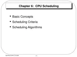
Chapter 6: CPU Scheduling • Basic Concepts • Scheduling Criteria • Scheduling Algorithms Operating System Concepts
Basic Concepts • Maximum CPU utilization obtained with multiprogramming. • CPU–I/O Burst Cycle • Process execution consists of a cycle of CPU execution and I/O wait. • Example: Alternating Sequence of CPU And I/O Bursts • In an I/O – bound program would have many very short CPU bursts. • In a CPU – bound program would have a few very long CPU bursts. Operating System Concepts
CPU Scheduler • The CPU scheduler (short-term scheduler) selects from among the processes in memory that are ready to execute, and allocates the CPU to one of them. • A ready queue may be implemented as a FIFO queue, priority queue, a tree, or an unordered linked list. • CPU scheduling decisions may take place when a process: 1. Switches from running to waiting state (ex., I/O request). 2. Switches from running to ready state (ex., Interrupts occur). 3. Switches from waiting to ready state (ex., Completion of I/O). 4. Terminates. • Scheduling under 1 and 4 is nonpreemptive; otherwise is called preemptive. • Under nonpreemptive scheduling, once the CPU has been allocated to a process, the process keeps the CPU until it releases the CPU either by terminating or by switching to the waiting state. Operating System Concepts
Dispatcher • Dispatcher module gives control of the CPU to the process selected by the short-term scheduler; this involves: • switching context • switching to user mode • jumping to the proper location in the user program to restart that program • Dispatch latency – time it takes for the dispatcher to stop one process and start another running. Operating System Concepts
Scheduling Criteria • CPU utilization – keep the CPU as busy as possible. • Throughput – number of processes that complete their execution per time unit. • Turnaround time – amount of time to execute a particular process; which is the interval from time of submission of a process to the time of completion (includes the sum of periods spent waiting to get into memory, waiting in ready queue, executing on the CPU, and doing I/O). • Waiting time – sum of the periods spent waiting in the ready queue. • Response time – the time from the submission of a request until the first response is produced (i.e., the amount of time it takes to start responding, but not the time that it takes to output that response). Operating System Concepts
Optimization Criteria • Max CPU utilization • Max throughput • Min turnaround time • Min waiting time • Min response time Operating System Concepts
Scheduling Algorithms • CPU scheduling deals with the problem of choosing a process from the ready queue to be executed by the CPU. • The following CPU scheduling algorithms will be described: • First-Come, First-Served (FCFS). • Shortest-Job-First (SJF). • Priority. • Round-Robin (RR). • Multilevel Queue. • Multilevel Feedback Queue. Operating System Concepts
Completion 3 2 1 CPU Ready Queue First-Come, First-Served (FCFS) Scheduling • It is the simplest CPU scheduling algorithm. • The process that requests the CPU first is allocated the CPU first. • The average waiting time under FCFS is long. Operating System Concepts
P1 P2 P3 0 24 27 30 First-Come, First-Served (FCFS) Scheduling • Example: ProcessBurst Time (milliseconds) P1 24 P2 3 P3 3 • Suppose that the processes arrive in the order: P1 , P2 , P3 The Gantt Chart for the schedule is: • Waiting time for P1 = 0; P2 = 24; P3 = 27 • Average waiting time: (0 + 24 + 27) / 3 = 17 (milliseconds) Operating System Concepts
P2 P3 P1 0 3 6 30 FCFS Scheduling (Cont.) Suppose that the processes arrive in the order P2 , P3 , P1 . • The Gantt chart for the schedule is: • Waiting time for P1 = 6;P2 = 0; P3 = 3 • Average waiting time: (6 + 0 + 3) / 3 = 3 (milliseconds) • Much better than previous case. • The order of processes in FCFS queue is important. Operating System Concepts
FCFS Scheduling (Cont.) • Another example, assume you have one CPU-bound process and many I/O-bound processes. • CPU executes the CPU-bound process and I/O-bound processes in ready queue after they used I/O devices (waiting). • So, I/O devices are idle. • All I/O-bound processes have very short CPU bursts. • The FCFS algorithm is nonpreemptive (i.e., the CPU keeps the process until either terminating or requesting I/O). Operating System Concepts
Shortest-Job-First (SJF) Scheduling • Associate with each process the length of its next CPU burst. Use these lengths to schedule the process with the shortest time. • Two schemes: • Nonpreemptive – once CPU given to the process it cannot be preempted until completes its CPU burst. • Preemptive – if a new process arrives with CPU burst length less than remaining time of current executing process, preempt. This scheme is known as the Shortest-Remaining-Time-First (SRTF). • If two processes have the same length next CPU burst, FCFS scheduling is used. • SJF is optimal – gives minimum average waiting time for a given set of processes. Operating System Concepts
P1 P3 P2 P4 0 3 7 8 12 16 Example of Non-Preemptive SJF • Example: ProcessArrival TimeBurst Time P1 0.0 7 P2 2.0 4 P3 4.0 1 P4 5.0 4 • SJF (non-preemptive) • Average waiting time = (0 + 6 + 3 + 7) / 4 = 4 Operating System Concepts
Example of Non-Preemptive SJF (Cont.) • If we used FCFS, then the average waiting time would be: (0 + 5 + 7 + 7) / 4 = 4.75 • The SJF gives less average waiting time than FCFS. • The SJF is a nonpreemptive in which the waiting process with the smallest estimated run-time-to-completion is run next. Therefore, SJF is not useful in timesharing environments. • Both FCFS and SJF are not useful for timesharing environments, because they are nonpreemptive. Operating System Concepts
P1 P2 P3 P2 P4 P1 11 16 0 2 4 5 7 Example of Preemptive SJF • Example: ProcessArrival TimeBurst Time P1 0.0 7 P2 2.0 4 P3 4.0 1 P4 5.0 4 • SJF (preemptive) [Shortest-Remaining-Time-First (SRTF)] • Average waiting time = (9 + 1 + 0 +2) / 4 = 3 Operating System Concepts
Priority Scheduling • A priority number (integer) is associated with each process. • The CPU is allocated to the process with the highest priority (smallest integer highest priority). • Equal priority processes are scheduled in FCFS. • SJF is a special case of general priority scheduling, where priority is the predicted next CPU burst time. • Priorities can be defined either internally or externally. • Internally use of some measurable quantity or quantities to compute the priority of a process. For example, memory requirements, number of open files, ratio of average I/O burst to average CPU burst have been used in computing priorities. • Externally priority is set by criteria that is external to the O.S.; such as importance of the process. Operating System Concepts
Priority Scheduling (Cont.) • Priority can be either preemptive or nonpreemptive. • A preemptive priority will preempt the CPU if the newly arrived process is higher than the priority of the currently running process. • A nonpreemptive priority will simply put the new highest priority process at the head of the ready queue. • Problem Starvation – low priority processes may never execute. • Solution Aging – as time progresses increase the priority of the process, so eventually the process will become the highest priority and will gain the CPU (i.e., the more time is spending a process in ready queue waiting, its priority becomes higher and higher). Operating System Concepts
P2 P5 P3 P4 P1 19 0 18 1 6 16 Example of Nonpreemptive Priority ProcessBurst TimePriority P1 10 3 P2 1 1 P3 2 3 P4 1 4 P5 5 2 • Gantt Chart: • Average waiting time = (0 + 1 + 6 + 16 + 18) / 5 = 8.2 Operating System Concepts
Ready Queue 3 2 1 Completion CPU Preemption Round Robin (RR) • The Round Robin is designed for time sharing systems. • The RR is similar to FCFS, but preemption is added to switch between processes. • Each process gets a small unit of CPU time (time quantum or time slice ), usually 10-100 milliseconds. After this time has elapsed, the process is preempted and added to the end of the ready queue. That is, after the time slice is expired an interrupt will occur and a context switch. Time Slice Operating System Concepts
Round Robin (Cont.) • If there are n processes in the ready queue and the time quantum is q, then each process gets 1/n of the CPU time in chunks of at most q time units at once. No process waits more than (n-1)q time units. • The performance of RR depends on the size of the time slice q : • If q very large (infinite) FIFO • If q very small RR is called processor sharing, and context switch increases. So, q must be large with respect to context switch, otherwise overhead is too high. Operating System Concepts
P1 P2 P3 P4 P1 P3 P4 P1 P3 P3 0 20 37 57 77 97 117 121 134 154 162 Example: RR with Time Quantum = 20 ProcessBurst TimeWaiting Time of each Process P1 53 0+(77-20)+(121-97)=81 P2 17 20 P3 68 37+(97-57)+(134-117)=94 P4 24 57+(117-77)=97 • The Gantt chart is: • Average Waiting Time = (81+20+94+97) / 4 = 73 Operating System Concepts
How a Smaller Time Quantum Increases Context Switches Operating System Concepts
Multilevel Queue • Ready queue is partitioned into separate queues: • foreground (interactive) • background (batch) • Each queue has its own scheduling algorithm: • foreground – RR • background – FCFS • Scheduling must be done between the queues. • Fixed priority scheduling; i.e., serve all from foreground then from background. Possibility of starvation. • Time slice – each queue gets a certain amount of CPU time which it can schedule amongst its processes; • 80% to foreground in RR • 20% to background in FCFS Operating System Concepts
Multilevel Queue Scheduling Operating System Concepts
Multilevel Feedback Queue • A process can move between various queues; aging can be implemented this way. • If a process waits too long in a lower-priority queue may be moved to a higher-priority queue (this form of aging to prevent starvation). • If a process uses too much CPU time, it will be moved to lower-priority queues. This leaves I/O bound and interactive processes in the higher-priority queues. • In general, the multilevel feedback queue scheduling algorithm is the most complex. Operating System Concepts
Multilevel Feedback Queues Operating System Concepts
Example of Multilevel Feedback Queue • Three queues: • Q0 – time quantum 8 milliseconds • Q1 – time quantum 16 milliseconds • Q2 – FCFS • Scheduling: • A new job enters queue Q0which is servedFCFS. When it gains CPU, job receives 8 milliseconds. If it does not finish in 8 milliseconds, job is moved to queue Q1. • At Q1 job is again served FCFS and receives 16 additional milliseconds. If it still does not complete, it is preempted and moved to queue Q2. • The Multilevel Feedback Queue Scheduling is preemptive. Operating System Concepts