Download
1 / 26
260 likes | 431 Views
CLIMARES – possible contributions from ECF and other partners to socio-economic modeling of the Arctic regions Klaus Hasselmann, Max Planck Insitute of Meteorology and ECF. Four main strands of socio-economic modeling: Agent-based, system dynamic models (ECF, MADIAMS)

E N D
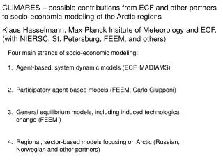
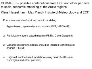
CLIMARES – possible contributions from ECF and other partners to socio-economic modeling of the Arctic regions Klaus Hasselmann, Max Planck Insitute of Meteorology and ECF • Four main strands of socio-economic modeling: • Agent-based, system dynamic models (ECF, MADIAMS) • Participatory agent-based models (FEEM, Carlo Giupponi) • General equilibrium models, including induced technological change (FEEM ) • Regional, sector-based models focusing on Arctic (Russian, Norwegian and other partners)
CLIMARES – possible contributions from ECF and other partners to socio-economic modeling of the Arctic regions Klaus Hasselmann, Max Planck Insitute of Meteorology and ECF • Four main strands of socio-economic modeling: • Agent-based, system dynamic models (ECF, MADIAMS) New modeling trend, but exists so far only in global version • Participatory agent-based models (FEEM, Carlo Giupponi) • Experience in regional applications (river basin areas), but not yet in larger areas such as Arctic • 3. General equilibrium models, including induced technological change (FEEM) • Reduced credibility through global financial crisis and recession, but important as reference to main stream • 4. Regional, sector-based models focusing on Arctic (Russian, Norwegian and other partners) • Essential for bringing all strands together
CLIMARES – possible contributions from ECF and other partners to socio-economic modeling of the Arctic regions • Four main strands of socio-economic modeling: • Agent-based, system dynamic models (ECF, MADIAMS) New modeling trend, but exists so far only in global version • Participatory agent-based models (FEEM, Carlo Giupponi) • Experience in regional applications (river basin areas), but not yet in larger areas such as Arctic • 3. General equilibrium models, including induced technological change (FEEM ?) • Reduced credibility through global financial crisis and recession, but important as reference to main stream • 4. Regional, sector-based models focusing on Arctic (Russian, Norwegian and other partners) • Essential for bringing all strands together
Traditional coupled climate-economic (integrated assessment-IA) model climate policy regulatory instruments scenario predictions ghg emissions climate system economic system impacts on production,welfare,…
Traditional coupled climate-economic (integrated assessment-IA) model climate policy regulatory instruments scenario predictions ghg emissions climate system economic system impacts on production,welfare,… “invisible hand“ establishes market equilibrium
MADIAM (Multi-Actor Dynamic Integrated Assessment Model) climate policy regulatory instruments Actors: governments, public, media, consumers, firms, workers, … scenario predictions ghg emissions climate system economic system impacts on production,welfare,… Dynamic evolution, governed by agent strategies
The “real economy”: Production output in physical units (Vensim diagram)
The “real economy”: Production output in physical units (Vensim diagram) y: total production , invested in: k: physical capital h: human capital g: consumer goods and services
The “virtual economy” (financial system): money circulation between firms, banks and households
Extensions to analyze impact of climate policies • Governments, with policies for carbon taxes, subsidies and recycling of tax income • Investment strategies: capital investments subdivided into fossil and renewable energies and energy efficiency • Consumer preferences for climate friendly and climate hostile goods • Assessment of climate change damages
Model M3a. Relative demand Good1(climate-friendly)/Good2(climate-hostile)
Model M3a.mitigation measures: w: weak, m: moderate, s: strong (a) (b)
Is climate change mitigation affordable? 4 - 3 - 1% BAU growth 2 - GDP (log Scale) 1 - 2100 2000
Is climate change mitigation affordable? 4 - 3 - 1% BAU growth 2 - BSP (log Skala) 1% GDP loss corresponds to a delay of 1 year over a period of 100 years–an affordable insurance premium to avoid the risk of dangerous climate change! (see also Azar and Schneider,2002) 1 - 2100 2000
Extensions to analyze impact of climate change in Arctic: • Include instabilities related to actor behaviour (e.g. financial crisis, business cycles, investment booms and busts)
Textbook view of equilibrium in supply and demand in relation to price (Samuelson and Nordhaus)
System dynamics representation of supply-demand-price interdependence dS/dt = F (S,D,P) (S = supply) dD/dt = G (S,D,P) (D = demand) dP/dt = H (S,D,P) (P = price)
System dynamics representation of supply-demand-price interdependence dS/dt = F (S,D,P) (S = supply) dD/dt = G (S,D,P) (D = demand) dP/dt = H (S,D,P) (P = price) • General result: A system of three first-order ordinary differential equations can have solutions representing: • a damped periodic, monotonic or non-monotonic (e.g. boom-bust) transition to an equilibrium point • a stable convergence to a periodic attractor • an unstable trajectory diverging to infinity • a bounded, non-periodic chaotic trajectory • Which type of solution is realized depends on the initial conditions and the behaviour of the economic actors
General equilibrium model: evolution to joint equilibrium in supply, demand and price for four different initial conditions
Boom-bust model: Equilibrium model:
Business cycle model: two-feedback loops, one postive (unstable),one negative (stabilizing) consumption decrease delcons positive loop production decrease dely increase negative loop wage decrease delw employm. increase demand supply price
Extensions to analyze impact of climate change in Arctic: • Include instabilities related to actor behaviour (e.g. financial crisis, business cycles, investment booms and busts) • Regionalization: different countries, different geographic regions • Sector resolution: different economic sectors (fishing, transportation, resources, tourism) • Feedbacks of consumer behaviour • Assessment of climate change damages • Uncertainty and risk assessment
Strategy: Develop hierarchy of models with gradually increasing complexity
Strategy: Develop hierarchy of models with gradually increasing complexity And apply Occam’s razor: use the simplest model that explains the phenomenon!