FACTORIAL DESIGNS

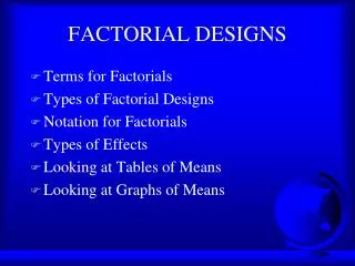
1. FACTORIAL DESIGNS • What is a factorial design? • Why use it? • When should it be used?

2. FACTORIAL DESIGNS • What is a factorial design? Two or more ANOVA factors are combined in a single study: eg. Treatment (experimental or control) and Gender (male or female). Each combination of treatment and gender are present as a group in the design.

3. FACTORIAL DESIGNS • Why use it? • In social science research, we often hypothesize the potential for a specific combination of factors to produce effects different from the average effects- thus, a treatment might work better for girls than boys. This is termed an INTERACTION

4. FACTORIAL DESIGNS • Why use it? • Power is increased for all statistical tests by combining factors, whether or not an interaction is present. This can be seen by the Venn diagram for factorial designs

6. FACTORIAL DESIGN • When should it be used? • Almost always in educational and psychological research when there are characteristics of subjects/participants that would reduce variation in the dependent variable, aid explanation, or contribute to interaction

7. TYPES OF FACTORS • FIXED- all population levels are present in the design (eg. Gender, treatment condition, ethnicity, size of community, etc.) • RANDOM- the levels present in the design are a sample of the population to be generalized to (eg. Classrooms, subjects, teacher, school district, clinic, etc.)

8. Factor B B 1 2 4 Factor A 1 A A 2 Two-dimensional representation of 2 x 4 factorial design GRAPHICALLY REPRESENTING A DESIGN B3 B4 B2 B3

9. Factor B 1 Factor 3 A 1 C A 1 A 2 Factor C Factor A 1 A C 2 A 2 Table 10.1: Two-dimensional representation of 2 x 4 factorial design Three-dimensional representation of 2 x 4 x3 factorial design GRAPHICALLY REPRESENTING A DESIGN B1 B4 B2 B3

10. LINEAR MODEL yijk =  + i + j + ij + eijk where  = population mean for populations of all subjects, called the grand mean, i = effect of group i in factor 1 (Greek letter nu), j = effect of group j in factor 2 (Greek letter omega), ij = effect of the combination of group i in factor 1 and group j in factor 2, eijk = individual subject k’s variation not accounted for by any of the effects above

11. Interaction Graph Suzy’s predicted score; she is in E Effect of being in Experimental group y Effect of being a girl Effect of being a girl in Experimental group mean Effect of not being a girl in Experimental group Effect of being a boy 0 Effect of being in Control group

12. y y level 2 of Factor K level 1 of M M Factor K E E A A N N S S level 2 of level 1 of Factor K Factor K L L L L L L 1 2 3 1 2 3 Factor L Factor L Ordinal Interaction Disordinal Interaction Fig. 10.4: Graphs of ordinal and disordinal interactions INTERACTION

13. 20 M E 15 A N S 10 Boys 5 Girls 0 Treatment 1 Treatment 2 Gender Disordinal interaction for 2 x 2 treatment by gender design INTERACTION

14. ANOVA TABLE • SUMMARY OF INFORMATION: SOURCE DF SS MS F E(MS) Independent Degrees Sum of Mean Fisher Expected mean variable of freedom Squares Square statistic square (sampling or factor theory)

15. PATH DIAGRAM • EACH EFFECT IS REPRESENTED BY A SINGLE DEGREE OF FREEDOM PATH • IF THE DESIGN IS BALANCED (EQUAL SAMPLE SIZE) ALL PATHS ARE INDEPENDENT • EACH FACTOR HAS AS MANY PATHS AS DEGREES OF FREEDOM, REPRESENTING POC’S

16. A 1 e A ijk 2 B y 1 ijk B 2 AB 2,2 AB 1,1 AB AB 1,2 2,1 : SEM representation of balanced factorial 3 x 3 Treatment (A) by Ethnicity (B) ANOVA

17. Contrasts in Factorial Designs • Contrasts on main effects as in 1 way ANOVA: POCs or post hoc • Interaction contrasts are possible: are differences between treatments across groups (or interaction within part of the design) significant? eg. Is the Treatment-control difference the same for Whites as for African-Americans (or Hispanics)? • May be planned or post hoc

18. C T 1 C T R 2 y.T T y y e e ijk ijk ijk ijk G 1 R R y.G y.TG G C TG TxG 1 C TG 2 Generalized effect path diagram Orthogonal contrast path diagram Two path diagrams for a 3 x 2 Treatment by Gender balanced factorial design

19. UNEQUAL GROUP SAMPLE SIZES • Unequal sample sizes induce overlap in the estimation of sum of squares, estimates of treatment effects • No single estimate of effect or SS is correct, but different methods result in different effects • Two approaches: parameter estimates or group mean estimates

20. UNEQUAL GROUP SAMPLE SIZES • Proportional design: main effects sample sizes are proportional: • Experimental-Male n=20 • Experimental-Female n=30 • Control- Male n=10 • Control-Female n=15 • Disproportional: no proportionality across cells M F E C 20 30 10 15

21. SST T SST T SSe e SSGT TG SSe e SSG G SSTG SSG TG G Unbalanced factorial design Unbalanced factorial design with proportional marginal sample sizes Venn diagrams for disproportional and proportional unbalanced designs

22. ASSUMPTIONS • NORMALITY • Robust with respect to normality and skewness with equal sample sizes, simulations may be useful in other cases • HOMOGENEOUS VARIANCES • problem if unequal sample sizes: small groups with large variances cause high Type I error rates • INDEPENDENT ERRORS: subjects’ scores do not depend on each other • always a problem if violated in multiple testing

23. GRAPHING INTERACTIONS • Graph means for groups: • horizontal axis represents one factor • construct separate connected lines for each crossing factor group • construct multiple graphs for 3 way or higher interactions

24. GRAPHING INTERACTIONS O u t c o m e females males c e1 e2 Treatment groups

25. EXPECTED MEAN SQUARES • E(MS) = expected average value for a mean square computed in an ANOVA based on sampling theory • Two conditions: null hypothesis E(MS) and alternative hypothesis E(MS) • null hypothesis condition gives us the basis to test the alternative hypothesis contribution (effect of factor or interaction)

26. EXPECTED MEAN SQUARES • 1 Factor design: Source E(MS) Treatment A 2e + n2A error 2e (sampling variation) Thus F=MS(A)/MS(e) tests to see if Treatment A adds variation to what might be expected from usual sampling variability of subjects. If the F is large, 2A  0.

27. EXPECTED MEAN SQUARES • Factorial design (AxB): SourceE(MS) Treatment A 2e + (1-b/B)n2AB + nb2A error 2e (sampling variation) Thus F=MS(A)/MS(e) does not test to see if Treatment A adds variation to what might be expected from usual sampling variability of subjects unless b=B or 2AB = 0 . If b (number of levels in study) = B (number in the population, factor is FIXED; else RANDOM

28. EXPECTED MEAN SQUARES • Factorial design (AxB): SourceE(MS) Treatment A 2e + (1-b/B)n2AB + nb2A AxB 2e + (1-b/B)n2AB error 2e (sampling variation) If 2AB = 0 , and B is random, then F = MS(A) / MS(AB) gives the correct test of the A effect.

29. EXPECTED MEAN SQUARES • Factorial design (AxB): SourceE(MS) Treatment A 2e + (1-b/B)n2AB + nb2A AB 2e + (1-b/B)n2AB error 2e (sampling variation) If instead we test F = MS(AB)/MS(e) and it is nonsignificant, then 2AB = 0 and we can test F = MS(A) / MS(e) *** More power since df= a-1, df(error) instead of df = a-1, (a-1)*(b-1)

30. Source df Expected mean square 2 2 2 s s s A (fixed) I-1 + n + nJ e AB A 2 2 s s B (random) J-1 + nI e B 2 2 s s AB (I-1)(J-1) + n e AB 2 s error N-IJK e Table 10.5: Expected mean square table for I x J mixed model factorial design

31. Mixed and Random Design Tests • General principle: look for denominator E(MS) with same form as numerator E(MS) without the effect of interest: F = 2effect + other variances /other variances • Try to eliminate interactions not important to the study, test with MS(error) if possible

32. NOTE: SPSS tests parameter effects, not mean effects; thus, SCHOOL should be tested with MS(SCHOOL)/MS(Error), which gives F=1.532, df=1,40, still not significant

33. PLOT OF INTERACTION OF SCHOOL AND PROGRAM ON SOCIAL SKILLS