Download
1 / 14
180 likes | 488 Views
Introduction to runoff modeling on the North Slope of Alaska using the Swedish HBV Model. Emily Youcha , Douglas Kane. University of Alaska Fairbanks Water & Environmental Research Center PO Box 755860 Fairbanks, AK 99775.

E N D
Introduction to runoff modeling on the North Slope of Alaska using the Swedish HBVModel Emily Youcha, Douglas Kane University of Alaska Fairbanks Water & Environmental Research Center PO Box 755860 Fairbanks, AK 99775
Use existing meteorological datasets and develop HBV model parameters to simulate runoff in both small and large North Slope Basins Objective Kavik Kuparuk Sag Upper Kuparuk
Approach • Begin runoff simulations on North Slope streams with abundance of data • Imnaviat Cr, 2.2 km2 (1985-present) • Upper Kuparuk River, 146 km2 (1993-present) • Putuligayuk River, 417 km2 (1970-1979, 1982-1986, 1999-2007) • Kuparuk River, 8140 km2 (1971-present) • Develop parameter sets and apply to other rivers (ungauged?)
HBV Model • Rainfall-runoff model, commonly used for forecasting in Sweden • Developed by Swedish Meteorological and Hydrological Institute • Semi-distributed conceptual model • Divide into sub-basins • Precipitation and temperature may be spatially distributed by applying areal-based weights to station data • Use of elevation and vegetation zones • Required data inputs (hourly or daily) include: • Precipitation (maximum end-of-winter SWE and summer precipitation) • Air temperature • Evapotranspiration (pan evaporation or estimated) daily or monthly • Routines include: • Snow • Soil Moisture Accounting • Response • Transformation
Snow Routine Inputs: Precipitation, Temperature Outputs: Snowpack, Snowmelt Soil Moisture Routine Inputs: Potential Evapotranspiration, Precipitation, Snowmelt Outputs: Actual Evapotranspiration, Soil Moisture, Ground-Water Recharge Response Routine Input: Ground-Water Recharge/Excess soil moisture Output: Runoff, Ground-Water Levels Transformation Routine Input: Runoff Simulated Runoff HBV Routines and Input Data SMHI
Soil Moisture Routine recharge Response Routine Q0=K0 * (SZ- UZL0) UZL0 SZ Q1=K1 * (SZ- UZL1) UZL1 Q2=K3 * SZ Recharge: input from soil routine (mm/day) SZ: Storage in zone (mm) UZL:Threshold parameter Ki: Recession coefficient (/day) Qi: Runoff component (mm/day) Runoff Modified from Siebert, 2005 SMHI Manual, 2005 SMHI Manual, 2005 Soil Moisture Routine Transformation Routine SMHI Manual, 2005 Routines and Parameters: Snow: 4 + parameters Degree-day method: Snowmelt = CFMAX * (T –TT) CFMAX=melting factor (mm/C-day) TT=threshold temperature (C) (snow vs. rain) CFR=refreezing factor to refreeze melt water WHC=water-holding capacity of snow (meltwater is retained in snowpack until it exceeds the WHC) Soil Moisture Accounting : 3+ parameters Modified bucket approach Shape coefficient (BETA) controls the contribution to the response function (runoff ratio) Limit of potential evapotranspiration (LP), the soil moisture value above which ET reaches Potential ET Maximum soil moisture (FC) Response 4+ parameters Transforms excess water from soil moisture zone to runoff. Includes both linear and non-linear functions. Upper reservoirs represent quickflow, lower reservoir represent slow runoff (baseflow). Lakes are considered as part of the lower reservoir. Lower reservoir may not be used (PERC parameter is set to zero due to presence of continuous permafrost). Transformation/Routing To obtain the proper shape of the hydrograph, parameter= MAXBAS (/d) Transformation Routine
HBV Calibration • Each model routine has parameters requiring model calibration • over 20 parameters, and may be varied throughout the simulated period (i.e. spring vs. summer) • Explained variance (observed vs. simulated) is the Nash-Sutcliffe (1970) model efficiency criterion good model fit is R-efficiency=1. Also looked at accumulative volume difference and visually inspect the hydrograph. • Used the commercially available HBV software to manually calibrate the model by trial and error • We tried HBV automated calibration to estimate parameters (Monte Carlo procedure using “HBV-light” by Siebert, 1997). Produced many different parameter sets that would solve the problem. Many parameters were not well defined • Most of the time, model validation results not very good.
Observed Hydrographs for Imnaviat and Upper Kuparuk: 1996, 1999, 2002, 2005
Preliminary Automated Calibration Results (Monte Carlo Procedure) Dotty plots – look for parameters that are well defined
Automated Calibration Results (Monte Carlo Procedure) Snowmelt 2002Snowmelt Parameters
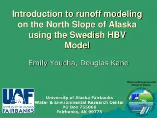
Summary • Need an automated calibration procedure to develop unique parameter sets • For Upper Kuparuk, model generally predicted timing of events (onset of snowmelt and timing of peak events). When it did not predict the proper timing, the model efficiency was poor. • For Upper Kuparuk, model overpredicted snowmelt flow volume and underpredicted extreme peak runoff events during summer • For both Upper Kuparuk and Imnavait, model did not predict the magnitude of peak flow • Problems may be attributed to not using a long enough simulation period • Many improvements are needed to increase the Nash-Sutcliffe model efficiency