Data Analysis Overview
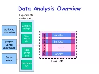
Different experiments. Data Analysis Overview. Experimental environment. prototype real sys. Workload parameters. Samples. exec- driven sim. System Config parameters. Samples. trace- driven sim. Samples. Factor levels. Raw Data. stochastic sim. Data Analysis Overview.

Data Analysis Overview
E N D
Presentation Transcript
Different experiments . . . Data Analysis Overview Experimentalenvironment prototype real sys Workloadparameters Samples exec-drivensim SystemConfigparameters Samples ... trace-drivensim Samples Factorlevels Raw Data stochasticsim
Data Analysis Overview • Comparison of Alternatives • Common case – one sample • point for each. • Conclusions only about this set of experiments. Experimentalenvironment prototype real sys Workloadparameters exec-drivensim SystemConfigparameters Repeated set 1 set of experiments . . . trace-drivensim Factorlevels Raw Data stochasticsim
Characterizing this sample data set • Central tendency – means, mode, median • Variability – range, std dev, COV, quantiles • Fit to known distribution • Sample data vs.Population • Confidence interval for mean • Significance level a • Sample size ngiven !r% accuracy Data Analysis Overview Experimentalenvironment prototype real sys Workloadparameters 1 repeated experiment exec-drivensim SystemConfigparameters Samples ... trace-drivensim Samples Factorlevels Raw Data stochasticsim
Comparison of Alternatives • Paired Observations • As one sample of pairwise differences ai - bi • Confidence interval A B . . . Data Analysis Overview Experimentalenvironment prototype real sys Workloadparameters 1 experiment exec-drivensim SystemConfigparameters Samples 1 set of experiments ... trace-drivensim Samples Factorlevels Raw Data stochasticsim
Unpaired Observations • As multiple samples, sample means and overlapping CIs • t-test on mean difference: xa - xb xb , sb ,CIb xa , sa ,CIa . . . Data Analysis Overview Experimentalenvironment prototype real sys Workloadparameters 1 experiment exec-drivensim SystemConfigparameters Samples 1 set of experiments ... trace-drivensim Samples Factorlevels Raw Data stochasticsim
y1y2yn Data Analysis Overview Experimentalenvironment • Regression models • response var = f (predictors) prototype real sys Workloadparameters Samples of response exec-drivensim Predictorvalues x,factor levels SystemConfigparameters Samples ... . . . trace-drivensim Samples Factorlevels Raw Data stochasticsim
Linear Regression Models • What is a (good) model? • Estimating model parameters • Allocating variation (R2) • Confidence intervals for regressions • Verifying assumptions visually
Confidence Intervals for Regressions • Regression is done from a single sample (size n) • Different sample might give different results • True model is y = 0 + 1x • Parameters b0 and b1 are really means taken from a population sample
Calculating Intervalsfor Regression Parameters • Standard deviations of parameters: • Confidence intervals are bi tsbi • where t has n - 2 degrees of freedom !
Example of Regression Confidence Intervals • Recall se = 0.13, n = 5, x2 = 264, = 6.8 • So • Using a 90% confidence level, t0.95;3 = 2.353
0.35 2.353(0.16) = (-0.03,0.73) ! Regression Confidence Example, cont’d • Thus, b0 interval is • Not significant at 90% • And b1 is • Significant at 90% (and would survive even 99.9% test) 0.29 2.353(0.004) = (0.28,0.30) !
Confidence Intervalsfor Predictions • Previous confidence intervals are for parameters • How certain can we be that the parameters are correct? • Purpose of regression is prediction • How accurate are the predictions? • Regression gives mean of predicted response, based on sample we took
N ymp S Predicting m Samples • Standard deviation for mean of future sample of m observations at xpis • Note deviation drops as m • Variance minimal at x = • Use t-quantiles with n–2 DOF for interval
N yp 2.67 2.353(0.14) = (2.34, 3.00) ! S Example of Confidenceof Predictions • Using previous equation, what is predicted time for a single run of 8 loops? • Time = 0.35 + 0.29(8) = 2.67 • Standard deviation of errors se = 0.13 • 90% interval is then
Other Regression Methods • Multiple linear regression – more than one predictor variable • Categorical predictors – some of the predictors aren’t quantitative but represent categories • Curvilinear regression – nonlinear relationship • Transformations – when errors not normally distributed or variance not constant • Handling outliers • Common mistakes in regression analysis
Multiple Linear Regression • Models with more than one predictor variable • But each predictor variable has a linear relationship to the response variable • Conceptually, plotting a regression line in n-dimensional space, instead of 2-dimensional
Basic Multiple Linear Regression Formula • Response y is a function of k predictor variables x1,x2, . . . , xk y = b0 + b1x1 + b2x2 + . . . + bkxk + e
. . . . . . . . . A Multiple Linear Regression Model Given sample of n observations model consists of n equations (note typo in book): . . . . . . . . . . . .
Looks Like It’s Matrix Arithmetic Time y = Xb +e . . . . . . . . .
Analysis ofMultiple Linear Regression • Listed in box 15.1 of Jain • Not terribly important (for our purposes) how they were derived • This isn’t a class on statistics • But you need to know how to use them • Mostly matrix analogs to simple linear regression results
Example ofMultiple Linear Regression • Internet Movie Database keeps popularity ratings of movies (in numerical form) • Postulate popularity of Academy Award winning films is based on two factors - • Age • Running time • Produce a regression rating = b0 + b1(length) +b2(age)
Some Sample Data Title Age Length Rating Silence of the Lambs 5 118 8.1 Terms of Endearment 13 132 6.8 Rocky 20 119 7.0 Oliver! 28 153 7.4 Marty 41 91 7.7 Gentleman’s Agreement 49 118 7.5 Mutiny on the Bounty 61 132 7.6 It Happened One Night 62 105 8.0
Now for Some Tedious Matrix Arithmetic • We need to calculate X, XT, XTX, (XTX)-1, and XTy • Because • We will see that b = (8.373, .005, -.009 ) • Meaning the regression predicts: rating = 8.373 + 0.005*age – 0.009*length
How Good Is ThisRegression Model? • How accurately does the model predict the rating of a film based on its age and running time? • Best way to determine this analytically is to calculate the errors or
Calculating the Errors, Continued • So SSE = 1.08 • SSY = • SS0 = • SST = SSY - SS0 = 452.9- 451.5 = 1.4 • SSR = SST - SSE = .33 • In other words, this regression stinks
Why Does It Stink? • Let’s look at the properties of the regression parameters • Now calculate standard deviations of the regression parameters
Calculating STDEVof Regression Parameters • Estimations only, since we’re working with a sample • Estimated stdev of
b0 = 8.37 (2.015)(1.29) = (5.77, 10.97)b1 = .005 (2.015)(.01) = (-.02, .02)b2 = -.009 (2.015)(.008) = (-.03, .01) ! ! ! Calculating Confidence Intervals • At the 90% level, for instance • Confidence intervals for • Only b0 is significant, at this level
Analysis of Variance • So, can we really say that none of the predictor variables are significant? • Not yet; predictors may be correlated • F-test can be used for this purpose • E.g., to determine if the SSR is significantly higher than the SSE • Equivalent to testing that y does not depend on any of the predictor variables
Running an F-Test • Need to calculate SSR and SSE • From those, calculate mean squares of the regression (MSR) and the errors (MSE) • MSR/MSE has an F distribution • If MSR/MSE > F-table, predictors explain a significant fraction of response variation • Note typos in book’s table 15.3 • SSR has k degrees of freedom • SST matches
F-Test for Our Example • SSR = .33 • SSE = 1.08 • MSR = SSR/k = .33/2 = .16 • MSE = SSE/(n-k-1) = 1.08/(8 - 2 - 1) = .22 • F-computed = MSR/MSE = .76 • F[90; 2,5] = 3.78 (at 90%) • So it fails the F-test at 90% (miserably)
Multicollinearity • If two predictor variables are linearly dependent, they are collinear • Meaning they are related • And thus the second variable does not improve the regression • In fact, it can make it worse • Typical symptom is inconsistent results from various significance tests
Finding Multicollinearity • Must test correlation between predictor variables • If it’s high, eliminate one and repeat the regression without it • If the significance of regression improves, it’s probably due to collinearity between the variables
Is Multicollinearity a Problem in Our Example? • Probably not, since the significance tests are consistent • But let’s check, anyway • Calculate correlation of age and length • After tedious calculation, -.25 • Not especially correlated • Important point - adding a predictor variable does not always improve a regression
Why Didn’t RegressionWork Well Here? • Check the scatter plots • Rating vs. age • Rating vs. length • Regardless of how good or bad regressions look, always check the scatter plots
Regression WithCategorical Predictors • Regression methods discussed so far assume numerical variables • What if some of your variables are categorical in nature? • Use techniques discussed later in the class if all predictors are categorical • Levels - number of values a category can take
HandlingCategorical Predictors • If only two levels, define bi as follows • bi = 0 for first value • bi = 1 for second value • This definition is missing from book in section 15.2 • Can use +1 and -1 as values, instead • Need k-1 predictor variables for k levels • To avoid implying order in categories
Categorical Variables Example • Which is a better predictor of a high rating in the movie database, winning an Oscar,winning the Golden Palm at Cannes, or winning the New York Critics Circle?
Choosing Variables • Categories are not mutually exclusive • x1= 1 if Oscar 0 if otherwise • x2= 1 if Golden Palm 0 if otherwise • x3= 1 if Critics Circle Award 0 if otherwise • y = b0+b1 x1+b2 x2+b3 x3
A Few Data Points Title Rating Oscar Palm NYC Gentleman’s Agreement 7.5 X X Mutiny on the Bounty 7.6 X Marty 7.4 X X X If 7.8 X La Dolce Vita 8.1 X Kagemusha 8.2 X The Defiant Ones 7.5 X Reds 6.6 X High Noon 8.1 X
And Regression Says . . . • How good is that? • R2 is 34% of the variation • Better than age and length • But still no great shakes • Are the regression parameters significant at the 90% level?