Download
1 / 34
340 likes | 477 Views
Distributed Algorithms – 2g1513. Lecture 1b – by Ali Ghodsi Models of distributed systems continued and logical time in distributed systems. State transition system - example. Example algorithm: Using graphs: X:=0; while (X<3) do X = X + 1; endwhile X:=1 Formally:

E N D
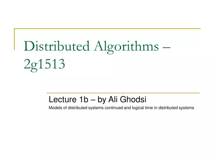
Distributed Algorithms – 2g1513 Lecture 1b – by Ali Ghodsi Models of distributed systems continued and logical time in distributed systems
State transition system - example • Example algorithm: Using graphs: X:=0; while (X<3) do X = X + 1; endwhile X:=1 • Formally: • States {X0, X1, X2} • Possible transitions {X0→X1, X1→X2, X2→X1} • Start states {X0} X1 start X0 X2
State transition system - formally A STS is formally described as the triple: (C, → , I) Such that: • C is a set of states • → is a subset of C C, describing the possible transitions (→ C C) • I is a subset of C describing the initial states (I C) Note that the system may have several transitions from one state E.g. → = {X2→X1, X2→X0}
Local Algorithms • The local algorithm will be modeled as a STS, in which the following three events happen: • A processor changes state from one state to a another state (internal event) • A processor changes state from one state to a another state, and sends a message to the network destined to another processor (send event) • A processor receives a message destined to it and changes state from one state to another (receive event)
Model of the distributed system • Based on the STS of a local algorithm, we can now define for the whole distributed system: • Its configurations • We want it to be the state of all processes and the network • Its initial configurations • We want it to be all possible configurations where every local algorithm is in its start state and an empty network • Its transitions, and • We want each local algorithm state event (send, receive, internal) be a configuration transition in the distributed system
Execution Example 1/9 • Lets do a simple distributed application, where a client sends a ping, and receives a pong from a server • This is repeated indefinitely p1 client send<ping, p2> send<pong, p1> p2 server
Execution Example 2/9 • M = {pingp2, pongp1} • (Zp1, Ip1, ├Ip1,├Sp1,├Rp1) • Zp1 ={cinit, csent} • Ip1 ={cinit} • ├Ip1 = • ├Sp1 ={(cinit, pingp2, csent)} • ├Rp1 ={(csent, pongp1, cinit)} • (Zp2, Ip2, ├Ip2,├Sp2,├Rp2) • Zp2 ={sinit, srec} • Ip2 ={sinit} • ├Ip2 = • ├Sp2 ={(srec, pongp1, sinit)} • ├Rp2 ={(sinit, pingp2, srec)} p1 client send<ping, p2> send<pong, p1> p2 server
Execution Example 3/9 • p1 (client) • (Zp1, Ip1, ├Ip1,├Sp1,├Rp1) • Zp1={cinit, csent} • Ip1={cinit} • ├Ip1= • ├Sp1={(cinit, pingp2, csent)} • ├Rp1={(csent, pongp1, cinit)} • p2 (server) • (Zp2, Ip2, ├Ip2,├Sp2,├Rp2) • Zp2={sinit, srec} • Ip2={sinit} • ├Ip2= • ├Sp2={(srec, pongp1, sinit)} • ├Rp2={(sinit, pingp2, srec)} C={ (cinit, sinit, ), (cinit, srec, ), (csent, sinit, ), (csent, srec, ), (cinit, sinit, {pingp2}), (cinit, srec, {pingp2}), (csent, sinit, {pingp2}), (csent, srec, {pingp2}), (cinit, sinit, {pongp1}), (cinit, srec, {pongp1}), (csent, sinit, {pongp1}), (csent, srec, {pongp1}) ...} I = { (cinit, sinit, ) } →={ (cinit, sinit, ) → (csent, sinit, {pingp2}), (csent, sinit, {pingp2}) → (csent, srec, ), (csent, srec, ) → (csent, sinit, {pongp1}), (csent, sinit, {pongp1}) → (cinit, sinit, )}
Execution Example 4/9 • p1 (client) • (Zp1, Ip1, ├Ip1,├Sp1,├Rp1) • Zp1={cinit, csent} • Ip1={cinit} • ├Ip1= • ├Sp1={(cinit, pingp2, csent)} • ├Rp1={(csent, pongp1, cinit)} • p2 (server) • (Zp2, Ip2, ├Ip2,├Sp2,├Rp2) • Zp2={sinit, srec} • Ip2={sinit} • ├Ip2= • ├Sp2={(srec, pongp1, sinit)} • ├Rp2={(sinit, pingp2, srec)} I = { (cinit, sinit, ) } →={(cinit, sinit, ) → (csent, sinit, {pingp2}), (csent, sinit, {pingp2}) → (csent, srec, ), (csent, srec, ) → (csent, sinit, {pongp1}), (csent, sinit, {pongp1}) → (cinit, sinit, )} E=( (cinit, sinit, ) , (csent, sinit, {pingp2}), (csent, srec, ), (csent, sinit, {pongp1}), (cinit, sinit, ), (csent, sinit, {pingp2}), … ) p1 state: cinit p2 state: sinit
Execution Example 5/9 • p1 (client) • (Zp1, Ip1, ├Ip1,├Sp1,├Rp1) • Zp1={cinit, csent} • Ip1={cinit} • ├Ip1= • ├Sp1={(cinit, pingp2, csent)} • ├Rp1={(csent, pongp1, cinit)} • p2 (server) • (Zp2, Ip2, ├Ip2,├Sp2,├Rp2) • Zp2={sinit, srec} • Ip2={sinit} • ├Ip2= • ├Sp2={(srec, pongp1, sinit)} • ├Rp2={(sinit, pingp2, srec)} I = { (cinit, sinit, ) } →={(cinit, sinit, ) → (csent, sinit, {pingp2}), (csent, sinit, {pingp2}) → (csent, srec, ), (csent, srec, ) → (csent, sinit, {pongp1}), (csent, sinit, {pongp1}) → (cinit, sinit, )} E=( (cinit, sinit, ) , (csent, sinit, {pingp2}), (csent, srec, ), (csent, sinit, {pongp1}), (cinit, sinit, ), (csent, sinit, {pingp2}), … ) p1 state: cinit p2 state: sinit
Execution Example 6/9 • p1 (client) • (Zp1, Ip1, ├Ip1,├Sp1,├Rp1) • Zp1={cinit, csent} • Ip1={cinit} • ├Ip1= • ├Sp1={(cinit, pingp2, csent)} • ├Rp1={(csent, pongp1, cinit)} • p2 (server) • (Zp2, Ip2, ├Ip2,├Sp2,├Rp2) • Zp2={sinit, srec} • Ip2={sinit} • ├Ip2= • ├Sp2={(srec, pongp1, sinit)} • ├Rp2={(sinit, pingp2, srec)} I = { (cinit, sinit, ) } →={(cinit, sinit, ) → (csent, sinit, {pingp2}), (csent, sinit, {pingp2}) → (csent, srec, ), (csent, srec, ) → (csent, sinit, {pongp1}), (csent, sinit, {pongp1}) → (cinit, sinit, )} E=( (cinit, sinit, ) , (csent, sinit, {pingp2}), (csent, srec, ), (csent, sinit, {pongp1}), (cinit, sinit, ), (csent, sinit, {pingp2}), … ) p1 state: csent send<ping, p2> p2 state: sinit
Execution Example 7/9 • p1 (client) • (Zp1, Ip1, ├Ip1,├Sp1,├Rp1) • Zp1={cinit, csent} • Ip1={cinit} • ├Ip1= • ├Sp1={(cinit, pingp2, csent)} • ├Rp1={(csent, pongp1, cinit)} • p2 (server) • (Zp2, Ip2, ├Ip2,├Sp2,├Rp2) • Zp2={sinit, srec} • Ip2={sinit} • ├Ip2= • ├Sp2={(srec, pongp1, sinit)} • ├Rp2={(sinit, pingp2, srec)} I = { (cinit, sinit, ) } →={(cinit, sinit, ) → (csent, sinit, {pingp2}), (csent, sinit, {pingp2}) → (csent, srec, ), (csent, srec, ) → (csent, sinit, {pongp1}), (csent, sinit, {pongp1}) → (cinit, sinit, )} E=( (cinit, sinit, ) , (csent, sinit, {pingp2}), (csent, srec, ), (csent, sinit, {pongp1}), (cinit, sinit, ), (csent, sinit, {pingp2}), … ) p1 state: csent rec<ping, p2> p2 state: srec
Execution Example 8/9 • p1 (client) • (Zp1, Ip1, ├Ip1,├Sp1,├Rp1) • Zp1={cinit, csent} • Ip1={cinit} • ├Ip1= • ├Sp1={(cinit, pingp2, csent)} • ├Rp1={(csent, pongp1, cinit)} • p2 (server) • (Zp2, Ip2, ├Ip2,├Sp2,├Rp2) • Zp2={sinit, srec} • Ip2={sinit} • ├Ip2= • ├Sp2={(srec, pongp1, sinit)} • ├Rp2={(sinit, pingp2, srec)} I = { (cinit, sinit, ) } →={(cinit, sinit, ) → (csent, sinit, {pingp2}), (csent, sinit, {pingp2}) → (csent, srec, ), (csent, srec, ) → (csent, sinit, {pongp1}), (csent, sinit, {pongp1}) → (cinit, sinit, )} E=( (cinit, sinit, ) , (csent, sinit, {pingp2}), (csent, srec, ), (csent, sinit, {pongp1}), (cinit, sinit, ), (csent, sinit, {pingp2}), … ) p1 state: csent send<pong, p1> p2 state: sinit
Execution Example 9/9 • p1 (client) • (Zp1, Ip1, ├Ip1,├Sp1,├Rp1) • Zp1={cinit, csent} • Ip1={cinit} • ├Ip1= • ├Sp1={(cinit, pingp2, csent)} • ├Rp1={(csent, pongp1, cinit)} • p2 (server) • (Zp2, Ip2, ├Ip2,├Sp2,├Rp2) • Zp2={sinit, srec} • Ip2={sinit} • ├Ip2= • ├Sp2={(srec, pongp1, sinit)} • ├Rp2={(sinit, pingp2, srec)} I = { (cinit, sinit, ) } →={(cinit, sinit, ) → (csent, sinit, {pingp2}), (csent, sinit, {pingp2}) → (csent, srec, ), (csent, srec, ) → (csent, sinit, {pongp1}), (csent, sinit, {pongp1}) → (cinit, sinit, )} E=( (cinit, sinit, ) , (csent, sinit, {pingp2}), (csent, srec, ), (csent, sinit, {pongp1}), (cinit, sinit, ), (csent, sinit, {pingp2}), … ) p1 state: cinit rec<pong, p1> p2 state: sinit
Applicable events • Any internal evente=(c,d)├Ipiis said to be applicable in anconfigurationC=(cp1, …, cpi, …, cpn, M) if cpi=c • If eventeis applied, we gete(C)=(cp1, …, d, …, cpn, M) • Any send event e=(c,m,d)├Spiis said to be applicable in an configuration C=(cp1, …, cpi, …, cpn, M) if cpi=c • If event eis applied, we get e(C)=(cp1, …, d, …, cpn, M{m}) • Any receive event e=(c,m,d)├Rpiis said to be applicable in an configuration C=(cp1, …, cpi, …, cpn, M) if cpi=c and mM • If event e is applied, we get e(C)=(cp1, …, d, …, cpn, M-{m})
Order of events • The following theorem shows an important result: • The order in which two applicable events are executed is not important! • Theorem: • Let ep and eq be two events on two different processors p and q which are both applicable in configuration . Then ep can be applied to eq(), and eq can be applied to ep(). • Moreover, ep(eq()) = eq(ep() ).
Order of events • To avoid a proof by cases (3*3=9 cases) we represent all three event types in one abstraction • We let the quadtuple (c, X, Y, d) represent any event: • c is the initial state of the processor • X is a set of messages that will be received by the event • Y is a set of message that will be sent by the event • d is the state of the processor after the event • Examples: • (cinit, , {ping}, csent) represents a send event • (sinit, {pong}, , srec) represents a receive event • (c1r, , , c2) represents an internal event • Any such event ep=(c, X, Y, d), at p, is applicable in a state ={…, cp,…, M} if and only if cp=c and XM.
Order of events • Proof: • Let ep={c, X, Y, d} andeq={e, Z, W, f} and ={…, cp, …, cq,…, M} • As bothep andepare applicable in we know thatcp=c, cq=e, XM, andZM. • eq()={…, cp, …, f,…, (M-Z)W}, • cp is untouched and cp=c, and X (M-Z)WasXZ=, henceep is applicable in eq() • Similar argument to show that eq is applicable in ep()
Order of events • Proof: • Lets proof ep(eq()) = eq(ep() ) • eq()={…, cp, …, f,…, (M-Z)W} • ep(eq())={…, d, …, f,…, (((M-Z)W)-X)Y} • ep()={…, d, …, cq,…, (M-X)Y} • eq(ep())={…, d, …, f,…, (((M-X)Y)-Z)W} • (((M-Z)W)-X)Y = (((M-X)Y)-Z)W • Because XZ=, WX=, YZ= • Both LHS and RHS can be transformed to ((M W Y)-Z)-X
Exact order does not always matter • In two cases the theorem does not apply: • If p=q, i.e. when the events occur on different processes • They would not both be applicable if they are executed out of order • If one is a sent event, and the other is the corresponding receive event • They cannot be both applicable • In such cases, we say that the two events are causally related!
Causally Order • The relation≤H on the events of an execution, called causal order, is defined as the smallest relation such that: • If e occurs before f on the same process, then e ≤H f • If s is a send event and r its corresponding receive event, then s ≤H r • ≤H is transitive. • I.e. If a ≤H b and b ≤H c then a ≤H c • ≤H is reflexive. • I.e. If a ≤H a for any event a in the execution • Two events, a and b, are concurrentiff a ≤H b and b ≤H a holds
Example of Causally Related events Concurrent Events Causally Related Events Time-space diagram p1 p2 p3 time Causally Related Events
Equivalence of Executions: Computations • Computation Theorem: • Let E be an execution E=(1, 2, 3…), and V be the sequence of events V=(e1, e2, e3…) associated with it • I.e. applying ek(k )=k+1 for all k≥1 • A permutation P of V that preserves causal order, and starts in 1, defines a unique execution with the same number of events, and if finite, P and V’s final configurations are the same • P=(f1, f2, f3…)preserves the causal order ofVwhen for every pair of eventsfi ≤H fj implies i<j
Equivalence of executions • If two executions F and E have the same collection of events, and their causal order is preserved, F and E are said to be equivalent executions, written F~E • F and E could have different permutation of events as long as causality is preserved!
Computations • Equivalent executions form equivalence classes where every execution in class is equivalent to the other executions in the class. • I.e. the following always holds for executions: • ~ is reflexive • I.e. If a~a for any execution • ~ is symmetric • I.e. If a~b then b~a for any executions a and b • ~ is transitive • If a~b and b~c, then a~c, for any executions a, b, c • Equivalence classes are called computations of executions
p1 p2 p3 time Example of equivalent executions • All three executions are part of the same computation, as causality is preserved Same color ~ Causally related p1 p2 p3 time p1 p2 p3 time
Two important results (1) • The computation theorem gives two important results • Result 1: • There is no distributed algorithm which can observe the order of the sequence of events (that can “see” the time-space diagram) • Proof: • Assume such an algorithm exists. Assume process p knows the order in the final configuration • Run two different executions of the algorithm that preserve the causality. • According to the computation theorem their final configurations should be the same, but in that case, the algorithm cannot have observed the actual order of events as they differ
Two important results (2) • Result 2: • The computation theorem does not hold if the model is extended such that each process can read a local hardware clock • Proof: • Similarly, assume a distributed algorithm in which each process reads the local clock each time a local event occurs • The final configuration of different causality preserving executions will have different clock values, which contradicts the computation theorem
Lamport Logical Clock (informal) • Each process has a local logical clock, which is kept in a local variable p for process p, which is initially 0 • The logical clock is updated for each local event on process p such that: • If an internal or send event occurs: • p =p+1 • If a receive event happens on a message from process q: • p = max(p, q)+1 • Lamport logical clocks guarantee that: • If a≤Hb, then p≤q, • where a and be happen on p and q
Example of equivalent executions p1 0 1 2 3 4 p2 0 4 5 p3 0 1 6 time
Vector Timestamps: useful implication • Each process p keeps a vector vp[n] of n positions for system with n processes, initially vp[p]=1 and vp[i]=0 for all other i • The logical clock is updated for each local event on process p such that: • If any event: • vp [p]=vp [p]+1 • If a receive event happens on a message from process q: • vp [x]= max(vp[x], vq[x]), for 1≤x≤n • We say vp≤vq y iff vp[x]≤vq[x] for 1≤x≤n • If not vp≤vq and not vq≤vp then vp is concurrent with vq • Lamport logical clocks guarantee that: • If vp≤vq then a≤Hb, and a≤Hb, then vp≤vq, • where a and be happen on p and q
Example of Vector Timestamps p1 [1,0,0] [2,0,0] [3,0,0] [4,0,0] [5,0,0] p2 [0,1,0] [4,2,0] [4,3,0] p3 [0,0,1] [0,0,2] [4,3,3] time This is great! But cannot be done with smaller vectors than size n, for n processes
Useful Scenario: what is most recent? p1 [1,0,0] [2,0,0] [3,0,0] [4,0,0] [5,0,0] p2 [5,2,0] [5,3,0] [0,1,0] p3 [0,0,1] [5,0,2] [5,0,3] time p2 examines the two messages it receives, one from p1 [4,0,0] and one from p2 [5,0,3] and deduces that the information from p1 is the oldest ([4,0,0]≤[5,0,3]).
Summary • The total order of executions of events is not always important • Two different executions could yield the same “result” • Causal order matters: • Order of two events on the same process • Order of two events, where one is a send and the other one a corresponding receive • Order of two events, that are transitively related according to above • Executions which contain permutations of each others event such that causality is preserved are called equivalent executions • Equivalent executions form equivalence classes called computations. • Every execution in a computation is equivalent to every other execution in its computation • Vector timestamps can be used to determine causality • Cannot be done with smaller vectors than size n, for n processes