Distributed k -ary System Algorithms for Distributed Hash Tables

1. Distributed k-ary SystemAlgorithms for Distributed Hash Tables Ali Ghodsi aligh@kth.se http://www.sics.se/~ali/thesis/ • PhD Defense, 7th December 2006, KTH/Royal Institute of Technology

2. Distributed k-ary SystemAlgorithms for Distributed Hash Tables Ali Ghodsi aligh@kth.se http://www.sics.se/~ali/thesis/ • PhD Defense, 7th December 2006, KTH/Royal Institute of Technology

3. Presentation Overview • Gentle introduction to DHTs • Contributions • The future

4. What’s a Distributed Hash Table (DHT)? • An ordinary hash table • Every node provides alookupoperation • Provide the value associated with a key • Nodes keeprouting pointers • If item not found, route to another node , which is distributed

5. So what? • Characteristic properties • Scalability • Number of nodes can be huge • Number of items can be huge • Self-manage in presence joins/leaves/failures • Routing information • Data items Time to find data is logarithmic Size of routing tables is logarithmic Example: log2(1000000)≈20 EFFICIENT! Store number of items proportional to number of nodes Typically: With D items and n nodes Store D/n items per node Move D/n items when nodes join/leave/fail EFFICIENT! • Self-management routing info: • Ensure routing information is up-to-date • Self-management of items: • Ensure that data is always replicated and available

6. Presentation Overview • … • … • What’s been the general motivation for DHTs? • … • …

7. Traditional Motivation (1/2) • Peer-to-Peer filesharing very popular • Napster • Completely centralized • Central server knows who has what • Judicial problems • Gnutella • Completely decentralized • Ask everyone you know to find data • Very inefficient central index decentralized index

8. Traditional Motivation (2/2) • Grand vision of DHTs • Provide efficient file sharing • Quote from Chord: ”In particular, [Chord] can help avoid single points of failure or control that systems like Napster possess, and the lack of scalability that systems like Gnutella display because of their widespread use of broadcasts.” [Stoica et al. 2001] • Hidden assumptions • Millions of unreliable nodes • User can switch off computer any time (leave=failure) • Extreme dynamism (nodes joining/leaving/failing) • Heterogeneity of computers and latencies • Unstrusted nodes

9. Our philosophy • DHT is a useful data structure • Assumptions might not be true • Moderate amount of dynamism • Leave not same thing as failure • Dedicated servers • Nodes can be trusted • Less heterogeneity • Our goal is to achieve more given stronger assumptions

10. Presentation Overview • … • … • How to construct a DHT? • … • …

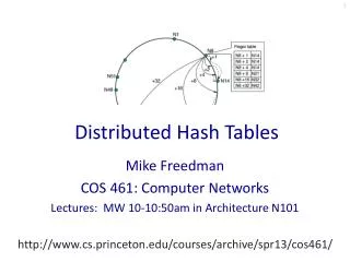
11. How to construct a DHT (Chord)? 0 15 1 14 2 13 3 12 4 5 11 6 10 7 9 8 • Use a logical name space, called the identifier space, consisting of identifiers {0,1,2,…, N-1} • Identifier space is a logical ring modulo N • Every node picks a random identifier • Example: • SpaceN=16 {0,…,15} • Five nodes a, b, c, d • a picks 6 • b picks 5 • c picks 0 • d picks 5 • e picks 2

12. Definition of Successor 0 15 1 14 2 13 3 12 4 5 11 6 10 7 9 8 • The successor of an identifier is the first node met going in clockwise direction starting at the identifier • Example • succ(12)=14 • succ(15)=2 • succ(6)=6

13. Where to store data (Chord) ? 0 15 1 14 2 13 3 12 4 5 11 6 10 7 9 8 • Use globally known hash function, H • Each item<key,value>gets identifierH(key) • Store each item at its successor • Node n is responsible for item k • Example • H(“Marina”)=12 • H(“Peter”)=2 • H(“Seif”)=9 • H(“Stefan”)=14 Store number of items proportional to number of nodes Typically: With D items and n nodes Store D/n items per node Move D/n items when nodes join/leave/fail EFFICIENT!

14. Where to point (Chord) ? 0 15 1 14 2 13 3 12 4 5 11 6 10 7 9 8 • Each node points to its successor • The successor of a node n is succ(n+1) • Known as a node’s succ pointer • Each node points to its predecessor • First node met in anti-clockwise direction starting at n-1 • Known as a node’s pred pointer • Example • 0’s successor is succ(1)=2 • 2’s successor is succ(3)=5 • 5’s successor is succ(6)=6 • 6’s successor is succ(7)=11 • 11’s successor is succ(12)=0

15. DHT Lookup 0 15 1 14 2 13 3 12 4 5 11 6 10 7 9 8 • To lookup a keyk • CalculateH(k) • Followsuccpointers untilitemkis found • Example • Lookup”Seif”at node 2 • H(”Seif”)=9 • Traverse nodes: • 2, 5, 6, 11 (BINGO) • Return “Stockholm” to initiator

16. Speeding up lookups 0 15 1 14 2 13 3 12 4 5 11 6 10 7 9 8 • If only pointer to succ(n+1) is used • Worst case lookup time is N, for N nodes • Improving lookup time • Point to succ(n+1) • Point to succ(n+2) • Point to succ(n+4) • Point to succ(n+8) • … • Point to succ(n+2M) • Distance always halved to the destination Time to find data is logarithmic Size of routing tables is logarithmic Example: log2(1000000)≈20 EFFICIENT!

17. Dealing with failures 0 15 1 14 2 13 3 12 4 5 11 6 10 7 9 8 • Each node keeps a successor-list • Pointer to fclosest successors • succ(n+1) • succ(succ(n+1)+1) • succ(succ(succ(n+1)+1)+1) • ... • If successor fails • Replace with closest alive successor • If predecessor fails • Set pred to nil

18. Handling Dynamism • Periodic stabilization used to make pointers eventually correct • Try pointing succ to closest alive successor • Try pointing pred to closest alive predecessor

19. Presentation Overview • Gentle introduction to DHTs • Contributions • The future

20. Outline • … • … • Lookup consistency • … • …

21. Problems with periodic stabilization • Joins and leaves can result in inconsistent lookup results • At node12, lookup(14)=14 • At node10, lookup(14)=15 12 14 15 10

22. Problems with periodic stabilization • Leaves can result in routing failures 13 16 10

23. Problems with periodic stabilization • Too many leaves destroy the system • #leaves+#failures/round < |successor-list| 12 14 11 15 10

24. Outline • … • … • Atomic Ring Maintenance • … • …

25. Atomic Ring Maintenance • Differentiate leaves from failures • Leave is a synchronized departure • Failure is a crash-stop • Initially assume no failures • Build a ring initially

26. Atomic Ring Maintenance • Separate parts of the problem • Concurrency control • Serialize neighboring joins/leaves • Lookup consistency

27. Naïve Approach • Each node ihosts a lock called Li • For p to join or leave: • First acquire Lp.pred • Second acquire Lp • Third acquire Lp.succ • Thereafter update relevant pointers • Can lead to deadlocks

28. Our Approach to Concurrency Control • Each node ihosts a lock called Li • For p to join or leave: • First acquire Lp • Thereafter acquire Lp.succ • Thereafter update relevant pointers • Each lock has a lock queue • Nodes waiting to acquire the lock

29. Safety • Non-interference theorem: • When node p acquires both locks: • Node p’s successor cannot leave • Node p’s ”predecessor” cannot leave • Other joins cannot affect ”relevant” pointers

30. Dining Philosophers • Problem similar to the Dining philosophers’ problem • Five philosophers around a table • One fork between each philosopher (5) • Philosophers eat and think • To eat: • grab left fork • then grab right fork

31. Deadlocks • Can result in a deadlock • If all nodes acquire their first lock • Every node waiting indefinitely for second lock • Solution from Dining philosophers’ • Introduce asymmetry • One node acquires locks in reverse order • Node with highest identifier reverses • If n<n.succ, then n has highest identity

32. Pitfalls • Join adds node/“philosopher” • Solution: some requests in the lock queue forwarded to new node 12 14 14, 12 12 12 14 15 10

33. Pitfalls • Leave removes a node/“philosopher” • Problem: if leaving node gives lock queue to its successor, nodes can get worse position in queue: starvation • Use forwarding to avoid starvation • Lock queue empty after local leave request

34. Correctness • Liveness Theorem: • Algorithm is starvation free • Also free from deadlocks and livelocks • Every joining/leaving node will eventually succeed getting both locks

35. Performance drawbacks • If many neighboring nodes leaving • All grab local lock • Sequential progress • Solution • Randomized locking • Release locks and retry • Liveness with high probability 12 14 15 10

36. Lookup consistency: leaves • So far dealt with concurrent joins/leaves • Look at concurrent join/leaves/lookups • Lookup consistency (informally): • At any time, only one node responsible for any key • Joins/leaves should “not affect” functionality of lookups

37. Lookup consistency • Goal is to make joins and leaves appear as if they happened instantaneously • Every leave has a leave point • A point in global time, where the whole system behaves as if the node instantaneously left • Implemented with a LeaveForward flag • The leaving node forwards messages to successor if LeaveForward is true

38. Leave Algorithm Node p Node q (leaving) Node r LeaveForward=true LeaveForward=false pred:=p succ:=r <LeavePoint, pred=p> <UpdateSucc, succ=r> <StopForwarding> leave point

39. Lookup consistency: joins • Every join has a join point • A point in global time, where the whole system behaves as if the node instantaneously joined • Implemented with a JoinForward flag • The successor of a joining node forwards messages to new node if JoinForward is true

40. Join Algorithm Node p Node q (joining) Node r Join Point JoinForward=true oldpred=pred pred=q JoinForwarding=false succ:=q pred:=p succ:=r <UpdatePred, pred=q> <JoinPoint, pred=p> <UpdateSucc, succ=q> <StopForwarding> <Finish>

41. Outline • … • … • What about failures? • … • …

42. Dealing with Failures • We prove it is impossible to provide lookup consistency on the Internet • Assumptions • Availability (always eventually answer) • Lookup consistency • Partition tolerance • Failure detectors can behave as if the networked partitioned

43. Dealing with Failures • We provide fault-tolerant atomic ring • Locks leased • Guarantees locks are always released • Periodic stabilization ensures • Eventually correct ring • Eventual lookup consistency

44. Contributions • Lookup consistency in presence of joins/leaves • System not affected by joins/leaves • Inserts do not “disappear” • No routing failures when nodes leave • Number of leaves not bounded

45. Related Work • Li, Misra, Plaxton (’04, ’06) have a similar solution • Advantages • Assertional reasoning • Almost machine verifiable proofs • Disadvantages • Starvation possible • Not used for lookup consistency • Failure-free environment assumed

46. Related Work • Lynch, Malkhi, Ratajczak (’02), position paper with pseudo code in appendix • Advantages • First to propose atomic lookup consistency • Disadvantages • No proofs • Message might be sent to a node that left • Does not work for both joins and leaves together • Failures not dealt with

47. Outline • … • … • Additional Pointers on the Ring • … • …

48. Routing • Generalization of Chord to provide arbitrary arity • Provide logk(n) hops per lookup • kbeing a configurable parameter • nbeing the number of nodes • Instead of only log2(n)

49. Achieving logk(n) lookup Node 0 I0 I1 I2 I3 Interval 3 Interval 0 Level 1 0…15 16…31 32…47 48…63 Interval 2 Interval 1 • Each node logk(N)levels, N=kL • Each level contains kintervals, • Example, k=4, N=64 (43), node 0 0 4 8 12 48 16 32

50. Achieving logk(n) lookup Interval 0 Node 0 Node 0 I0 I0 I1 I1 I2 I2 I3 I3 Interval 1 Level 1 Level 1 0…15 0…15 16…31 16…31 32…47 32…47 48…63 48…63 Interval 2 Level 2 0…3 4…7 8…11 12…15 Interval 3 • Each node logk(N)levels, N=kL • Each level contains kintervals, • Example, k=4, N=64 (43), node 0 0 4 8 12 48 16 32